Current trajectory image-based protection algorithm for transmission lines connected to MMC-HVDC stations using CA-CNN

Abstract

In the presence of an MMC-HVDC system, current differential protection (CDP) has the risk of failure in operation under an internal fault. In addition, CDP may also incur security issues in the presence of current transformer (CT) saturation and outliers. In this paper, a current trajectory image-based protection algorithm is proposed for AC lines connected to MMC-HVDC stations using a convolution neural network improved by a channel attention mechanism (CA-CNN). Taking the dual differential currents as two-dimensional coordinates of the moving point, the moving-point trajectories formed by differential currents have significant differences under internal and external faults. Therefore, internal faults can be identified using image recognition based on CA-CNN. This is improved by a channel attention mechanism, data augmentation, and adaptive learning rate. In comparison with other machine learning algorithms, the feature extraction ability and accuracy of CA-CNN are greatly improved. Various fault conditions like different network structures, operation modes, fault resistances, outliers, and current transformer saturation, are fully considered to verify the superiority of the proposed protection algorithm. The results confirm that the proposed current trajectory image-based protection algorithm has strong learning and generalizability, and can identify internal faults reliably.

1 Introduction

In recent years, modular multilevel converter-based high voltage direct current (MMC-HVDC) technology has been rapidly developed as a result of its modular structure, ease of manufacturing, independent control of reactive and active power, and low switching losses [1]. With these characteristics, it has broad application in long-distance power transmission, offshore wind power grid connection [2], asynchronous interconnection, and large capacity power transmission.

The fault current characteristics of MMC-HVDC are somewhat different from those of synchronous generators because of the high controllability and limited overcurrent capacity of an MMC-HVDC, so that conventional relaying protection schemes may operate incorrectly [3]. References [4,5,6] investigate the influence of VSC-HVDC on the distance protection of AC lines connected to it, but a corresponding solution is not provided. In [7], a zone I distance relaying protection scheme is proposed for the degradation of the distance protection performance caused by the integration of MMC-HVDC, one which can accurately identify internal faults. However, the proposed scheme cannot operate accurately under symmetrical faults. The authors in [8] propose a primary protection scheme based on improved distance protection and fiber-optic communication, which can operate correctly under all fault types. However, there are still some limitations, such as the inability to identify fault phases and slow operation in some cases. In [9], a pilot protection scheme based on the ratio of the currents on both terminals of the transmission line is proposed. Although it can identify faults of lines emanating from the VSC-HVDC system, it cannot identify the fault phase and has a high risk of maloperation under high-resistance faults. References [10,11,12,13] propose new current differential protection schemes for the AC lines connected to wind farms. However, different from wind farms, an MMC-HVDC station has both rectifier and inverter modes, so the proposed schemes in [10,11,12,13] may operate incorrectly in some cases. Additionally, the schemes in [10,11,12,13] do not have good tolerance against some nonideal conditions during an external fault, e.g., CT saturation and outliers. Reference [14] proposes an enhanced current differential protection scheme that has good performance in different operational modes of the MMC. However, two additional methods are introduced to eliminate the negative effects of CT saturation and outliers, considerably increasing the complexity of the protection scheme. Reference [15] puts forward time-domain pilot protection for lines connecting MMC-HVDC stations. However, its operating performance depends heavily on the reasonable selection of protection thresholds. Considering the rapid increase of the number and capacity of MMC-HVDC projects and the drawbacks of existing protection algorithms, it is imperative to have a new proposal for the protection of AC transmission lines connected to MMC-based converter stations. Given the rapid development of artificial intelligence and its wide application in various industries, using artificial intelligence to solve relay protection problems has become a new way of thinking.

Deep learning, as a representative of artificial intelligence techniques, has strong nonlinear fitting and feature expression ability. It can extract fault information from complex and multi-variable fault data. Therefore, in relay protection, artificial intelligence technology has broad application prospects. Reference [16] proposes a new method for transmission line fault detection and classification based on a convolutional sparse autoencoder, which has high accuracy of fault detection and classification. In [17], a method is presented for detection and classification of transient faults based on a graph convolutional neural network. However, the graph convolution is less flexible and cannot deal with dynamic grid structure. Reference [18] introduces a CNN-based fault classification method using the Hilbert-Huang transform to build the time-frequency energy matrix of the fault signal as the input matrix of the CNN. However, the datasets constructed by this method are too complex to be applied in practice. Reference [19] performs continuous wavelet transform on the zero-sequence current signal to obtain a time-frequency grayscale image. A method of faulty feeder detection based on CNN trained by grayscale images is proposed, while [20] proposes a fault location method based on an adaptive CNN. It has high fault recognition accuracy and fast convergence speed. Reference [21] measures the zero-sequence currents at both sides of the line to obtain the characteristic waveform, and uses a 1-D CNN for fault location. This does not require massive amounts of data for training. However, references [19,20,21] can only detect ground faults without considering other fault types. Most existing solutions that combine artificial intelligence with relay protection also choose to apply machine learning and deep learning to fault identification and detection, and the accuracy rate still needs to be improved. Specifically, the application of deep learning to the protection algorithm for AC lines connected to MMC-HVDC stations still needs to be studied in conjunction with the specific fault characteristics of MMC-based converter stations. Garnered from the literature review, the pros and cons of different protection schemes are summarized in Table 1.

Table 1 Pros and cons of existing protection schemes

The key contributions of this paper are:

• 1. The concept of current trajectory image is developed. The difference of current trajectory image under various fault conditions and nonideal conditions, including severe internal fault, high-resistance internal fault, external faults, CT saturation and outliers, is analyzed. The method of discriminating between internal and external faults by means of current trajectory image is introduced.

• 2. A protection algorithm based on image recognition of the differential current trajectory is proposed. A CNN is adopted for image recognition to distinguish between internal and external faults under different conditions.

• 3. To improve recognition accuracy, convergence speed, and robustness of the CNN, three improvement methods are introduced: channel attention mechanism, adaptive decay learning rate, and data augmentation. Compared with other advanced algorithms, e.g., KNN, decision tree, ANN, and CNN, CA-CNN has higher recognition accuracy and can identify internal faults reliably.

The rest of the paper is as follows: Sect. 2 describes the current trajectory image formed by differential currents, and analyzes the difference of current trajectory images between internal and external faults. Section 3 introduces the implementation steps of the current trajectory image-based protection algorithm and the improvement methods of CA-CNN. In Sect. 4, a simulation model is built to generate data sets, and the effectiveness and superiority of the proposed scheme are evaluated by comparing CA-CNN with other algorithms. Finally, the conclusions are summarized in Sect. 5.

2 Current trajectory image formed by dual differential currents

Different from traditional synchronous generators, the fault current of an MMC-HVDC system has a limited amplitude and controlled phase angle. This is attributed to the overcurrent capability of the fully controlled power electronic devices and the highly controllable characteristics of the converter station. Because of the above special fault characteristics, the traditional current differential protection algorithm may undergo performance degradation or even give incorrect operation in the presence of MMC-based converter stations [14]. In addition, some nonideal conditions during external faults, e.g., CT saturation and outliers, also negatively affect the security of the differential protection. Consequently, it is essential to propose a novel protection algorithm capable of replacing CDP for AC lines connected to the converter stations.

Differential current is defined as the summation of the currents on the grid side and the converter station side of a line. This includes all information about the fault currents on both sides of the transmission line. If the information of fault currents can be fully exploited, internal and external faults can be theoretically distinguished. The key to the matter is how to make adequate use of the current information, for which the method based on current trajectory images formed by dual differential currents is proposed to obtain information to identify internal faults.

2.1 Analysis of differential current waveforms

Figure 1 shows a simplified model of an AC grid connected with an MMC-HVDC station. The buses M and N represent the buses on the converter station side and grid side, respectively. i_m (I_m) and i_n (I_n) are the currents flowing to the line by bus M and bus N, respectively.

Fig. 1

Simplified model of AC grid connected with MMC-HVDC station

When internal faults occur in the AC line connected to an MMC-HVDC station, as illustrated in Fig. 1, the differential current i_d is composed of the fundamental frequency AC component and the decaying DC component [22], expressed as:

$$i_{d} = i_{n} + i_{m} = I_{ac} \cos (\omega_{0} t + \varphi_{ac} ) - I_{dc} e^{ - t/T}$$

(1)

In (1), I_ac is the amplitude of the fundamental frequency AC component, I_dc is the initial value of the decaying DC component, ω₀ is the fundamental frequency of the power grid, φ_ac denotes the initial phase angle, T represents the decaying time constant, which is inversely proportional to the fault resistance.

The decaying DC component is related to the fault resistance. The decaying time constant decreases as the fault resistance increases, and the DC component contained in the differential current also decreases. The waveforms of the differential current when there are internal faults with small and large fault resistances are shown by the black lines in Fig. 2.

Fig. 2

Waveforms of the differential current under internal faults. a Small fault resistance. b Large fault resistance

When external faults occur, the currents of the grid and the converter sides have equal amplitudes and opposite directions, and the differential current is approximately zero. The waveform of differential current under an external fault is shown by the black line in Fig. 3a. CT saturation can cause the measured differential current to deviate from zero. The black line in Fig. 3b shows the differential current waveform under an external fault with severe CT saturation.

Fig. 3

Waveforms of the differential current under external faults. a Without CT saturation. b With severe CT saturation

The CT saturation distorts the differential current. This should be approximately zero in the condition of external faults. If the amplitude of the differential current is taken as the criterion of relay protection, as is the case in CDP, CT saturation will seriously affect the judgment on the occurrence of external faults, potentially misidentifying external faults as internal.

2.2 Trajectory of the moving point constructed by differential currents

In order to fully exploit the information of the differential current, the differential current is delayed by 1/4 cycle as shown by the red dashed lines in Figs. 2 and 3. Taking the differential current $i_{d}$ and delayed differential current $i^{\prime}_{d}$ as two-dimensional coordinates of the moving point, the moving point $(i_{d} ,i^{\prime}_{d} )$ forms a trajectory, one which can efficiently differentiate between internal and external faults under various conditions, such as different fault resistances, types, locations, CT saturation, and outliers.

• 1. Internal Faults

When internal faults occur, the delayed differential current $i_{d}^{\prime }$ is given by [15]:

$$\begin{aligned} & i_{d}^{\prime } = i{}_{d}(t - \frac{{T_{0} }}{4}) \\ & \quad = I_{ac} \cos (\omega_{0} t - \omega_{0} \frac{{T_{0} }}{4} + \varphi_{ac} ) - I_{dc} e^{{ - (t - \frac{{T_{0} }}{4})/T}} \\ \end{aligned}$$

(2)

Usually, T > > T₀/4, ω₀T₀ = 2π, whereby the following relation can be obtained:

$$i_{d}^{\prime } \approx I_{ac} \sin (\omega_{0} t + \varphi_{ac} ) - I_{dc} e^{ - t/T}$$

(3)

Figure 4 shows the formation process of a moving-point trajectory formed by differential currents when internal faults occur.

Fig. 4

The formation process of moving-point trajectory formed by differential currents when internal faults occur

If the fault resistance is large, as shown in (1), the decaying DC component contained in the differential current is small and can be ignored. The differential current can be simplified as $i_{d} = I_{ac} \cos (\omega t)$. After a delay of 1/4 cycle, $i_{d}^{\prime } = I_{ac} \sin (\omega t)$. As shown by the green waveforms in Fig. 4, the time-varying cosine and sine signals are mapped to the x-axis and y-axis respectively, and the trajectory of the moving point $(i_{d} ,i_{d}^{\prime } )$ is a circle. The radius of the circle is determined by the amplitude I_ac of the sine and cosine signals. If the fault resistance is small, the decaying DC component cannot be ignored. The addition of the DC component offsets the center of the moving-point trajectory formed by the differential currents, as shown by the red waveforms in Fig. 4. As the DC component decays the center of the moving-point trajectory gradually approaches the origin.

• 2. External Faults

Under normal conditions or external faults, the differential current is approximately zero, so the trajectories of moving points constructed by differential currents in this case are concentrated near the origin. When $i_{d} \approx 0,i_{d}^{\prime } \ne 0$, the moving-point trajectory is on the y-axis, and when $i_{d} \ne 0,i_{d}^{\prime } \approx 0$, the moving-point trajectory is on the x-axis. As shown in Fig. 3b, for the condition of an external fault with severe CT saturation, the moving-point trajectory formed by differential currents is near the x-axis and y-axis, except for the period just after the fault occurrence, when both $i_{d}$ and $i_{d}^{\prime }$ are not equal to zero and the moving-point trajectory formed by differential currents is not near the x-axis nor y-axis.

Intercepting the moving-point trajectory formed by differential currents starting from T₀/4 after the fault occurrence and lasting for one power frequency period, the moving-point trajectories formed by differential currents under various conditions are shown in Fig. 5. Figure 5a–c show the trajectories of moving points constructed by differential currents under an internal fault, while Figs. 5d–f show the trajectories of moving points constructed by differential currents under an external fault.

Fig. 5

The trajectories of moving points constructed by differential currents under diverse conditions. a Internal fault with large fault resistance. b Internal fault with small fault resistance. c Internal fault with severe CT saturation. d External fault or the normal condition. e External fault with severe CT saturation. f External fault with outliers

According to the above analysis, there is a significant difference in the trajectories of moving points constructed by differential currents between internal and external faults. Therefore, it is feasible to fulfill the differentiation of internal and external faults by means of current trajectory image, and realize the appropriate operation of relays of AC lines connected to the MMC-based converter stations.

3 Current trajectory image-based protection algorithm

The current trajectory image-based protection algorithm using a convolutional neural network improved by channel attention mechanism (CA-CNN) proposed in this paper is shown in Fig. 6. The implementation steps of this algorithm can be summarized as follows.

• 1. Collect the current information at both ends of the line, and calculate the dual differential currents $i_{d}$ and $i_{d}^{\prime }$ to obtain the image of differential currents trajectory formed by moving point $(i_{d} ,i_{d}^{\prime } )$. The images are preprocessed by unifying the coordinate axis range and the image size, and are converted into grayscale images.

• 2. Consider a variety of different situations to generate data sets, design the model architecture of the CNN, normalize the data sets and divide them into the training set and test set, and then train the CNN to obtain the optimal model parameters.

• 3. After the model is trained, fault identification of unknown transmission lines can be carried out by feeding the normalized current trajectory images of the three phases to the CNN, to allow accurate differentiation between internal and external faults in addition to identifying the fault phases.

Fig. 6

The procedure of the proposed current trajectory image-based protection algorithm

3.1 Convolutional neural network

A CNN is a feedforward neural network, extensively used for its powerful feature extraction capability in the field of image recognition. Compared with machine learning algorithms, a CNN has three prominent features: sparse connectivity, parameter sharing, and down sampling. On the one hand, these features considerably decrease the network parameters and reduce the complexity of the model, and on the other, they further reduce the risk of overfitting, so a CNN offers a substantial benefit in two-dimensional image processing with good robustness and computational efficiency.

The CNN structure contains three main parts: convolution, pooling, and fully connected layers. The convolution layer realizes feature extraction through the convolution kernel. This is equivalent to a weight matrix, and the convolution kernel slides on the feature map with a fixed step size to realize local feature extraction. Different convolution kernels correspond to different local features.

The operation performed by each convolution kernel sliding on the feature map is:

$$x^{l} = f(W^{l} \cdot x^{l - 1} + b^{l} )$$

(4)

where l represents the number of layers, x^l represents the feature map matrix of the current layer, x^l−1 is the feature map matrix of the previous layer, W^l is the convolution kernel weight matrix, “·” represents the dot product operation, b represents the bias, and f() represents the excitation function.

Pooling is actually a down-sample process. The pooling layer is between consecutive convolutional layers and is used to reduce the number of parameters. This can improve operational speed and prevent overfitting while retaining useful information. The pooling method refers to using the overall statistical characteristics of the adjacent square regions to replace the output of that position, without increasing the parameters required for training. For example, max pooling indicates that the maximum value within adjacent square regions is taken as the output.

The fully connected layer unfolds the feature maps output from the convolution layer and pooling layer into a one-dimensional matrix that acts as “classifier” throughout the CNN. The two outputs represent the probability of the faults judged as internal and external faults respectively.

The training processes of the CNN are: first, the network parameters are initialized randomly, and then the training image is taken as the input to the CNN, to perform forward propagation operations of the convolution, pooling, and fully connected layers, and to calculate the corresponding output probability of each category. Finally, the error between output values and actual values is calculated, and all network parameters are updated by the gradient descent method to minimize the output error.

3.2 Improvement measures

To further improve the recognition accuracy, training speed and generalizability of the CNN, three measures are proposed: channel attention mechanism, adaptive decay learning rate, and data augmentation. The structure of the improved CNN (CA-CNN) for the current trajectory image-based protection algorithm is shown in Fig. 7. In Fig. 7, “FC” represents the fully-connected layer, “GAP” represents global average pooling, “f” represents the number of convolution kernels, and “s” represents the stride size.

Fig. 7

Structure of CA-CNN

• 1. Channel Attention Mechanism

An attention mechanism is added to boost the representational capabilities of the network and the accuracy of fault identification. The fundamental thought behind the attention mechanism is that the model learns to concentrate on important information and ignore inconsequential information [23, 24]. By learning the importance of each channel, the important features are weighted according to their importance, and the weight of unimportant features is reduced. This is called the channel attention mechanism.

Figure 8 shows the basic principle of the mechanism. The feature map is convolved with a convolution kernel to generate the first channel of the next layer. There are “f” convolution kernels, so the number of channels in the next layer is C₂, which is equal to f. The channel attention mechanism performs a weighting operation on the channels, learns the weights through the neural network, and increases the weights for important channels and reduces the weights for unimportant channels, corresponding to the depth of the color, as in Fig. 8. The channel of the next layer is related to the convolution kernel. Therefore, the channel attention mechanism is also equivalent to weighting the convolution kernel, evaluating the features extracted by each convolution kernel, adding weights to important features and reducing weights of unimportant features.

Fig. 8

The fundamental principle of the channel attention mechanism

For the specific channel attention model structure shown in Fig. 7, H, W, C represent the height, width, and channel of the feature map, respectively. Global average pooling (GAP) is to average each channel of the feature map [25], and change the size of the feature map from H × W × C to 1 × 1 × C while retaining the feature map information. The output of the previous layer is connected to the global average pooling and fully connected layers, and a sigmoid activation function to generate a 1 × 1 × C weight matrix. This is multiplied by the output of the previous layer to form the input of the next layer.

• 2. Adaptive Decay Learning Rate

The learning rate is one of the important hyperparameters for training neural networks, and determines how fast the network learns. During network training, the model gives predicted values through forward propagation, calculates the cost function and adjusts parameters through backpropagation. The above process is repeated so that the model parameters progressively approach the optimal solution and the optimal model is obtained. Within this process, the learning rate is the one in charge of controlling the step size of the process of parameter update.

If the learning rate is large, the parameter update speed will be very fast, which can achieve fast network convergence. However, if the learning rate is too large, it may lead the parameters to be updated in the wrong direction and consequently the cost function may explode instead of converge. If the learning rate is small, the network may not miss the optimal point, but the network will learn slowly. In addition, it may be trapped in a local optimum if the learning rate is too small.

An adaptive decay learning rate is thus proposed. Early in the training of the network, a relatively large learning rate will be selected to accelerate the convergence of the network. The learning rate then gradually decreases as the number of iterations increases to ensure that the network eventually converges to the global optimal solution, instead of oscillating or exploding in its vicinity. The formula for the learning rate α is given as:

$$\alpha = \left\{ {\begin{array}{*{20}l} {\alpha_{0} } \hfill & {epoch \le N} \hfill \\ {\alpha_{0} e^{0.2(N - epoch)} } \hfill & {epoch > N} \hfill \\ \end{array} } \right.$$

(5)

where α₀ indicates the initial learning rate.

According to (5), when the number of epochs is greater than N, the learning rate begins to decay. Faster convergence and higher accuracy can be achieved when setting N = 5.

• 3. Data Augmentation

Image classification relies on a large amount of labeled data to train the model, and the limitation of the data set size will bring problems such as overfitting and low generalizability of the model. Data augmentation uses limited data to generate numerous equivalent data, allowing for a greater number and diversity of training samples, and can improve the robustness of the model.

Using left-right translation and up-and-down translation to generate more equivalent data, this reduces overfitting and gives the resultant model stronger generalizability. The image of the dataset generated by simulation is in an ideal state. The actual collected image data is relatively fuzzy, and it is easy to identify errors. Adding noise to the training data can both enhance the robustness of the model and diminish the susceptibility of the model to image quality.

4 Performance evaluation

4.1 Data set

In order to construct a great deal of labeled data sets of current trajectory image required for deep learning, the IEEE 39-bus system with a 200 MW MMC-HVDC system is built in PSCAD/EMTDC, as shown in Fig. 9. The length of the transmission line 1–2 is 50 km, and the parameters can be found in [26, 27].

Fig. 9

The IEEE 39-bus system with a MMC-HVDC system

The current trajectory images are different under different fault conditions. A set of data is generated by fully considering the effects of different fault types, resistances, and locations, as well as different operational modes of the converter, CT saturation, and outliers. The specific parameters are shown in Table 2. As the data set fully considers various situations, the neural network can quickly learn useful information from a lot of data and improve the accuracy of fault identification.

Table 2 Conditions and parameters of the data set

A total of 3272 sample data are obtained from the simulated experiments by parameter traversal, and the data are randomly subdivided into a training set and a test set in the ratio of 8:2, i.e., the sizes of training and test sets are 2618 and 654, respectively.

4.2 CNN training and testing results

The CA-CNN structure is shown in Fig. 7, using adaptive decay learning rate with the initial value of α₀ = 0.01. The data set is fed into the CA-CNN and the CNN, and the training set is used to train the model. The test set is then used for testing the accuracy of the model to verify its validity.

The neural networks are trained and tested for 10 cycles on the 3272 dataset, and the results are shown in Fig. 10. When the epoch is 10, the accuracies of the CNN training set and test set are 98.97% and 99.07% respectively, while the accuracies of the CA-CNN training set and test set are 99.89% and 100%, respectively. The CA-CNN enhances the accuracy of the model while the convergence speed is significantly faster than that of the CNN. It is also found that the accuracy of the network increased rapidly in the early stages of training. When the epoch is 4, the accuracies of the training set and the test set both reach over 98%.

Fig. 10

Accuracy curves of CNN and CA-CNN

To investigate the effects of the three methods of attention mechanism, decay learning rate, and data augmentation on the CNN, the accuracies of the training and test sets are shown in Table 3 by combining each of these three methods with the CNN.

Table 3 The accuracy for the three methods added individually

As can be seen from Table 3, combining each of the three methods mentioned in SubSect. 3.2 with the CNN model alone, and the addition of all three methods increases the accuracy of the model compared to the simple CNN model.

4.3 Comparison of different algorithms

To evaluate the superiority of the CA-CNN, some existing machine learning algorithms such as K-Nearest Neighbor (KNN), Decision Tree, Artificial Neural Network (ANN) are compared with the CA-CNN. These methods are briefly described as follows.

• 1. The KNN algorithm uses the distance between samples to judge similarity. It calculates the distance between the unknown sample and all training samples, and obtains K training samples with the closest distance. If most of the K samples which are similar to the unknown sample belong to a certain category, the unknown sample also belongs to this category.

• 2. Decision tree is an algorithm that learns the classification rules in the data set through decisive features and divides the unknown data set. The decision tree is constructed by selecting features through information gain. In order to prevent overfitting, the decision tree needs to be pruned.

• 3. ANN refers to a network structure that consists of a massive number of interconnected neurons, which are used to simulate the organizational structure and operation mechanism of the brain. An ANN mainly involves input, hidden and output layers. This paper adopts an ANN structure with five hidden layers, and the numbers of neurons are 256, 128, 64 and 32, respectively.

We input the same training set and test set, and the test results of different algorithms are shown in Table 4.

Table 4 Comparison of different algorithms

As shown in Table 4, the proposed CA-CNN fault identification method has higher accuracy than KNN, Decision Tree and ANN. The results verify the effectiveness and superiority of the CA-CNN by extracting the information of the input data through multiple convolution layers.

The comparisons of different algorithms under different fault types, locations, and resistances are shown in Fig. 11.

Fig. 11

Comparison of different algorithms under different conditions. a Different fault types. b Different fault locations. c Different fault resistances. d Internal fault and external fault

As shown in Fig. 11a, different algorithms exhibit different fault identification accuracies under different fault types. KNN has the lowest accuracy and the CA-CNN has the highest accuracy. Similarly, the CA-CNN offers the highest fault identification accuracy under different fault locations and resistances.

Overall, comparing the recognition accuracy of different algorithms under internal and external faults, as shown in Fig. 11d, different algorithms have higher recognition accuracy for external faults. The CA-CNN performs well for both internal and external faults.

The results show that CA-CNN has stronger generalizability and higher accuracy than KNN, Decision Tree, ANN, and CNN under various fault conditions.

4.4 Comparison of CDP and Proposed Protection Algorithm

We refer to the current reference direction in Fig. 1. The criterion of current differential protection (CDP) for an internal fault can be given by:

$$\underbrace {{\left| {{\varvec{I}}_{{\text{m}}} + {\varvec{I}}_{{\text{n}}} } \right|}}_{operating\;current} > K\underbrace {{\left| {{\varvec{I}}_{{\text{m}}} - {\varvec{I}}_{{\text{n}}} } \right|}}_{restraining\;current}$$

(6)

where K is the restraint coefficient. I_m and I_n are the currents flowing to the line by bus M and bus N, respectively, while the bold font style represents a phasor.

If both ends of the AC transmission line are synchronous generators, during an internal fault, the phase difference of the fault currents on both sides is an acute angle. As a result, operating current surpasses restraining current, and CDP can identify internal fault reliably, as shown in Fig. 12a. However, when an MMC-based converter station is present and operates in rectifier mode, it is possible that the phase difference of the fault currents between the two sides of the AC line is an obtuse angle [14]. In this case, operating current may be lower than restraining current, causing CDP to have high probability of being ineffective, as shown in Fig. 12b.

Fig. 12

Spatial relationship of current phasors. a Acute angle. b Obtuse angle

When an external fault occurs, the phase angle difference between I_m and I_n approaches 180°, and their amplitudes are close to each other. In this condition, |I_m + I_n|≈0 and |I_m − I_n|≈|I_m| +|I_n|. Thus, |I_m + I_n| is remarkably less than K|I_m − I_n|, so CDP does not operate. However, the above analysis is no longer true in the presence of CT saturation. CT saturation results in serious distortion of secondary current, and consequently operating current has a high risk of exceeding restraining current, particularly for severe CT saturation. The false tripping signal may be generated and the situation is similar in the presence of outliers.

In summary, two issues should be focused on: 1) When internal faults occur, CDP may fail to operate particularly in the rectifier mode of the converter station; 2) When external faults occur, CDP may misoperate in the presence of CT saturation or outliers.

For the above two problems, the current trajectory image-based protection algorithm is compared with CDP, and simulations are carried out according to different conditions as shown in Table 5. The fault inception time is 2 s, and “√” and “ × ” in Table 5 represent correct and wrong identification results respectively.

Table 5 Comparison of CDP and proposed protection algorithm

The simulation waveforms of the 5 cases in Table 5 are displayed in Fig. 13, wherein the amplitude ratio represents |I_m + I_n|/|I_m − I_n|.

Fig. 13

Simulation results of CDP under different cases. a Case 1. b Case 2. c Case 3. d Case 4. e Case 5

Figure 13a-d show that CDP does not correctly identify the faults in these four cases. As can be seen in Fig. 13a, b, CDP may not operate under high fault resistance when internal faults occur, whereas Fig. 13c, d show that CDP may misoperate in the case of CT saturation and outliers when external faults occur.

The current trajectories images generated under the same conditions are shown in Fig. 14. The current trajectory images of each phase are fed into the trained CA-CNN separately for identification and all the current trajectory images are identified correctly. The results demonstrate that the proposed algorithm outperforms CDP in protecting the AC lines connected to MMC-based converter stations.

Fig. 14

The current trajectory images of the three-phase under different cases. a Case 1. b Case 2. c Case 3. d Case 4. e Case 5

4.5 Performance assessment under nonideal conditions

CT saturation, CT measurement errors, and capacitive currents may have a negative impact on the reliability of conventional protection schemes. To test the performance of the proposed current trajectory image-based protection algorithm under these nonideal conditions, the following three experiments are performed.

• (1) As described in Sect. 2.2, CT saturation distorts the differential current and thus affects the current trajectory image, and different severity of CT saturation needs to be considered. Setting different fault conditions and considering CT saturation of different severities, 144 simulations are performed in the system shown in Fig. 9, and a total of 432 current trajectory images of three phases are obtained and fed into the trained CA-CNN for testing. All the faults are correctly identified, and the results are compared with other machine learning algorithms in Fig. 16.

• (2) CT measurement errors cause the differential current under external faults to no longer close to zero, which in turn causes the current trajectory image under external faults to no longer concentrate at the origin, as shown in Fig. 15. Considering CT measurement errors of 3%, 6% and 10%, 432 current trajectory images are constructed and all of them are correctly identified by the CA-CNN model, and the results of comparison with other machine learning algorithms are shown in Fig. 16.

  Fig. 15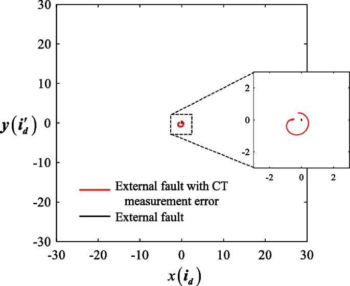

  

  The trajectory of moving points constructed by differential currents under external fault with CT measurement error

  Fig. 16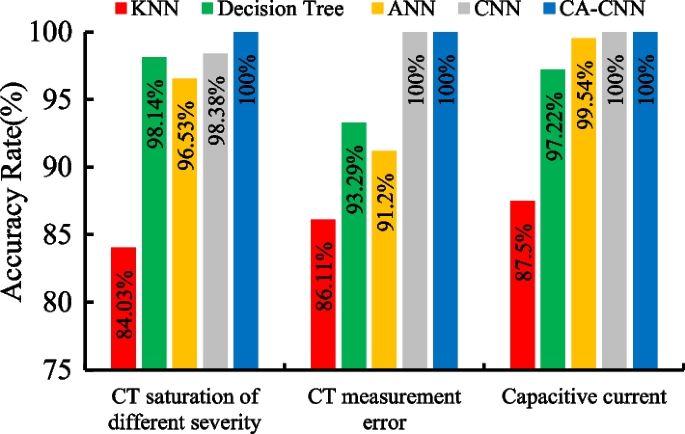

  

  Comparison of different algorithms under CT saturation of different severity, CT measurement, and capacitive current

• (3) Similar to CT measurement errors, capacitive currents may adversely affect conventional protection schemes. The capacitance current is changed by varying the transmission line length, and 432 current trajectory images are constructed by considering transmission line lengths of 100 km, 200 km and 300 km, all of which can be correctly identified by the CA-CNN. The results of comparison with other machine learning algorithms are also shown in Fig. 16.

As shown in Fig. 16, even in the nonideal cases of different CT saturation, CT measurement errors and capacitance currents, the CA-CNN still performs better than other algorithms, which fully demonstrates the superiority of the proposed protection scheme.

4.6 Active power reversal

An MMC-based converter station has two operational modes, i.e., rectifier and inverter. Reversal of power is realized in the simulation model. As shown in Fig. 17, the active power is gradually reversed from − 200 MW (− 1.0 pu) to 200 MW (1.0 pu). During power reversal, three internal faults are set at t = 2, 2.09 and 2.15 s. The three current trajectories corresponding to the three fault inception times are shown in Fig. 18.

Fig. 17

Active power waveform at converter station side

Fig. 18

The moving point trajectory under internal fault when the fault is set at: a 2 s. b 2.09 s. c 2.15 s

The current trajectory images are fed into the trained CA-CNN model, and all three images are identified correctly. This shows that the proposed protection algorithm can accurately identify the fault when power is reversed.

In the case of external faults, the currents flowing through the two ends of the line remain approximately equal in amplitude and 180° out of phase, and the differential current i_d approximately equals 0. The generated current trajectory images are concentrated near the origin and are not affected by the power reversal.

4.7 Performance test based on images constructed by data obtained from RTDS-based experimental system

To further validate the performance of the proposed current trajectory image-based protection algorithm, the RTDS-based experimental system shown in Fig. 19 is used. The MMC-HVDC model is built in RTDS based on the actual engineering parameters of the YuE interconnection MMC-HVDC project, while the actual control devices are used. The fault recorded data can be obtained from the RTDS-based experimental system. The length of the transmission line between the converter station and the grid is 100 km, the positive sequence impedance is (0.01839 + j0.263) Ω/km, and the zero sequence impedance is (0.1417 + j0.6027) Ω/km.

Fig. 19

Laboratory system built on RTDS and real control and protection equipment

The effectiveness of the proposed current trajectory image-based protection algorithm is confirmed by conducting experiments considering different fault conditions, and the results are shown in Table 6. The proposed protection scheme is tested for correct operation under internal faults by changing the fault type, fault location, fault resistance and operational mode. A total of 32 internal fault experiments are carried out, and the CA-CNN based protection algorithm correctly identifies all of them and distinguishes the fault phases. Compared with the ANN and CNN, the accuracy of the CA-CNN is significantly higher. At the same time, internal faults that cannot be identified by traditional CDP are correctly recognized by the proposed algorithm. Thirteen external fault experiments are conducted by changing the fault type and operational mode and considering severe CT saturation and outliers. The experiments show that the CA-CNN can correctly identify external faults, does not misoperate when external faults occur, and is not affected by CT saturation and outliers. This contrast with CDP which is easily affected by CT saturation and outliers in the case of external faults, and is prone to false operation. CDP is correct in not operating for only 7 out of the 13 external fault experiments, while the remaining 6 incorrect operations are all due to CT saturation and outliers.

Table 6 Comparison of different algorithm using RTDS

Communication delay leads to data un-synchronization, which has negative effect on the security of protection. Thus, the tolerance against communication delay is important for line protection. The communication delay in a fiber-optic cable is about 5 μs/km [28], so the delay for a 100 km transmission line is about 0.5 ms. To evaluate the tolerance of proposed protection against communication delay, a communication delay of 0.5 ms is considered in this paper.

The current trajectory images under external and internal faults with 0.5 ms communication delay are shown in Fig. 20. The current trajectory images are fed into the trained CA-CNN. The results are all correct, which shows that the proposed method is insensitive to the communication delay and can still correctly identify internal and external faults.

Fig. 20

The current trajectory images of communication delay in different cases. a External fault with 0.5 ms communication delay (fault type: ACG). b Internal fault with 0.5 ms communication delay (fault type: BC)

5 Conclusion

To address the problem that the presence of an MMC-HVDC station may lead to poor dependability of CDP under internal faults and incorrect operation under external faults, a current trajectory image-based protection algorithm using CA-CNN is proposed. The performance of the proposed scheme is thoroughly evaluated using PSCAD and RTDS. The main conclusions are:

• 1. The moving-point trajectories formed by taking the dual differential currents as two-dimensional coordinates of the moving points have significant differences between internal and external faults under different conditions. The CNN can accurately identify the images of moving-point trajectory and distinguish internal and external faults.

• 2. The feature extraction ability and convergence speed of a CNN are improved by introducing a channel attention mechanism, adaptive decay learning rate, and data augmentation. Compared with machine learning algorithms such as KNN, Decision Tree, and ANN, the accuracy of fault identification of the CA-CNN is superior.

• 3. The proposed current trajectory image-based protection algorithm performs well in discriminating accurately between internal and external faults in addition to identifying the fault phase. The algorithm demonstrates superb reliability and robustness, regardless of fault conditions and operational modes, and exhibits excellent performance even in the presence of CT saturation and outliers.

References

Nguyen, T. H., Hosani, K. A., & Moursi, M. S. E. (2019). Alternating submodule configuration based MMCs with carrier-phase-shift modulation in HVdc systems for dc-fault ride-through capability. IEEE Transactions on Industrial Informatics, 15(9), 5214–5224.
Yang, B., Liu, B., Zhou, H., Wang, J., Yao, W., Wu, S., Shu, H., & Ren, Y. (2022). A critical survey of technologies of large offshore wind farm integration: Summary, advances, and perspectives. Protection and Control of Modern Power Systems., 7(1), 17.
Quispe, J. C., & Orduña, E. (2022). Transmission line protection challenges influenced by inverter-based resources: A review. Protection and Control of Modern Power Systems., 7(1), 1–7.
Alam, M. M., Leite, H., Liang, J., & da Silva Carvalho, A. (2017). Effects of VSC based HVDC system on distance protection of transmission lines. International Journal of Electrical Power & Energy Systems., 92, 245–260.
Alam, M. M., Leite, H., Silva, N., & da Silva Carvalho, A. (2017). Performance evaluation of distance protection of transmission lines connected with VSC-HVDC system using closed-loop test in RTDS. Electric Power Systems Research., 152, 168–183.
Jia, K., Chen, R., Xuan, Z., Yang, Z., Fang, Y., & Bi, T. (2018). Fault characteristics and protection adaptability analysis in VSC-HVDC-connected offshore wind farm integration system. IET Renewable Power Generation, 12(13), 1547–1554.
Liang, Y., Li, W., & Huo, Y. (2021). Zone I distance relaying scheme of lines connected to MMC-HVDC stations during asymmetrical faults: Problems, challenges, and solutions. IEEE Transactions on Power Delivery, 36(5), 2929–2941.
Liang, Y., Huo, Y., & Zhao, F. (2021). An accelerated distance protection of transmission lines emanating from MMC-HVdc stations. IEEE Journal of Emerging and Selected Topics in Power Electronics, 9(5), 5558–5570.
Xue, S., Yang, J., Chen, Y., Wang, C., Shi, Z., Cui, M., & Li, B. (2016). The applicability of traditional protection methods to lines emanating from VSC-HVDC interconnectors and a novel protection principle. Energies, 9(6), 400–426.
Jia, K., Li, Y., Fang, Y., Zheng, L., Bi, T., & Yang, Q. (2018). Transient current similarity based protection for wind farm transmission lines. Applied Energy, 225, 42–51.
Zhang, L., Jia, K., Bi, T., Fang, Y., & Yang, Z. (2021). Cosine similarity based line protection for large scale wind farms. IEEE Transactions on Industrial Electronics, 68(7), 5990–5999.
Zhang, L., Jia, K., Wu, W., Liu, Q., Bi, T., & Yang, Q. (2021). Cosine similarity based line protection for large scale wind farms part II—the industrial application. IEEE Transactions on Industrial Electronics. doi:https://doi.org/10.1109/TIE.2021.3069400.
Saber, A., Shaaban, M. F., & Zeineldin, H. H. (2022). A new differential protection algorithm for transmission lines connected to large-scale wind farms. International Journal of Electrical Power & Energy Systems, 141, 108220.
Liang, Y., Ren, Y., & He, W. (2022). An enhanced current differential protection for AC transmission lines connecting MMC-HVDC stations. IEEE Systems Journal. https://doi.org/10.1109/JSYST.2022.3155881
Liang, Y., Ren, Y., & Zhang, Z. (2023). Pilot protection based on two-dimensional space projection of dual differential currents for lines connecting MMC-HVDC stations. IEEE Transactions on Industrial Electronics, 70(5), 4356–4368.
Chen, K., Hu, J., & He, J. (2018). Detection and classification of transmission line faults based on unsupervised feature learning and convolutional sparse autoencoder. IEEE Transactions on Smart Grid, 9(3), 1748–1758.
Tong, H., Qiu, R. C., Zhang, D., Yang, H., Ding, Q., & Shi, X. (2021). Detection and classification of transmission line transient faults based on graph convolutional neural network. CSEE Journal of Power and Energy Systems, 7(3), 456–471.
Guo, M., Yang, N., & Chen, W. (2019). Deep-learning-based fault classification using Hilbert-Huang transform and convolutional neural network in power distribution systems. IEEE Sensors Journal, 19(16), 6905–6913.
Guo, M., Zeng, X., Chen, D., & Yang, N. (2018). Deep-learning-based earth fault detection using continuous wavelet transform and convolutional neural network in resonant grounding distribution systems. IEEE Sensors Journal, 18(3), 1291–1300.
Liang, J., Jing, T., Niu, H., & Wang, J. (2020). Two-terminal fault location method of distribution network based on adaptive convolution neural network. IEEE Access, 8, 54035–54043.
Guo, M., Gao, J., Shao, X., & Chen, D. (2021). Location of single-line-to-ground fault using 1-D convolutional neural network and waveform concatenation in resonant grounding distribution systems. IEEE Transactions on Instrumentation and Measurement, 70, 1–9.
Sriharan, S., & De Oliveira, S. E. M. (1977). Analysis of synchronous generator sequential short circuits. Proceedings of the Institution of Electrical Engineers, 124(6), 549–553.
Guo, M. H., Xu, T. X., Liu, J. J., Liu, Z. N., Jiang, P. T., Mu, T. J., Zhang, S. H., Martin, R. R., Cheng, M. M., \& Hu, S. M. Attention mechanisms in computer vision: A survey. Computational Visual Media 8(3), 331–368.
Hu, J., Shen, L., Albanie, S., Sun, G., & Wu, E. (2020). Squeeze-and-excitation networks. IEEE Transactions on Pattern Analysis and Machine Intelligence, 42(8), 2011–2023.
Lin, M., Chen, Q., & Yan, S. (2014). Network in network. In International conference on learning representations, Banff, Canada.
Hiskens, I. IEEE PES task force on benchmark systems for stability controls, Tech. Rep., November 2013, [Online]. Available: http://www.sel.eesc.usp.br/ieee/
Manitoba Hydro International Ltd. IEEE 39 Bus System, IEEE 39 bus technical note, May. 2018, [Online]. Available:https://hvdc.ca/knowledge-base/read,article/28/ieee-39-bus-system/v
Farshad, M. (2021). A pilot protection scheme for transmission lines of half-bridge MMC-HVDC grids using cosine distance criterion. IEEE Transactions on Power Delivery, 36(2), 1089–1096.
Acknowledgements
This work was supported in part by the Fundamental Research Funds for the Central Universities under Grant 2022JCCXJD01, in part by Training Program of Innovation and Entrepreneurship for Undergraduates of China University of Mining and Technology (Beijing) under Grant 202204009.
Funding
None.
Author information
Authors and Affiliations
Contributions
YL: methodology, reviewing and editing, supervision. YR: methodology, investigation, software, writing-original draft preparation, validation. JY: software, validation. WZ: methodology, investigation. All authors read and approved the final manuscript.
Corresponding author
Ethics declarations
Competing interest
The authors declare that they have no known competing financial interests or personal relationships that could have appeared to influence the work reported in this paper.
Rights and permissions
Open Access This article is licensed under a Creative Commons Attribution 4.0 International License, which permits use, sharing, adaptation, distribution and reproduction in any medium or format, as long as you give appropriate credit to the original author(s) and the source, provide a link to the Creative Commons licence, and indicate if changes were made. The images or other third party material in this article are included in the article's Creative Commons licence, unless indicated otherwise in a credit line to the material. If material is not included in the article's Creative Commons licence and your intended use is not permitted by statutory regulation or exceeds the permitted use, you will need to obtain permission directly from the copyright holder. To view a copy of this licence, visit http://creativecommons.org/licenses/by/4.0/.
About this article
Cite this article
Liang, Y., Ren, Y., Yu, J. et al. Current trajectory image-based protection algorithm for transmission lines connected to MMC-HVDC stations using CA-CNN. Prot Control Mod Power Syst 8, 6 (2023). https://doi.org/10.1186/s41601-023-00280-3
Received:
Accepted:
Published:
DOI: https://doi.org/10.1186/s41601-023-00280-3