- Original research
- Open access
- Published:
Estimating zero-sequence impedance of three-terminal transmission line and Thevenin impedance using relay measurement data
Protection and Control of Modern Power Systems volume 3, Article number: 36 (2018)
Abstract
Current and voltage waveforms recorded by intelligent electronic devices (IEDs) are more useful than just performing post-fault analysis. The objective of this paper is to present techniques to estimate the zero-sequence line impedance of all sections of a three-terminal line and the Thevenin equivalent impedance of the transmission network upstream from the monitoring location using protective relay data collected during short-circuit ground fault events. Protective relaying data from all three terminals may not be always available. Furthermore, the data from each terminal may be unsynchronized and collected at different sampling rates with dissimilar fault time instants. Hence, this paper presents approaches which use unsynchronized measurement data from all the terminals as well as data from only two terminals to estimate the zero-sequence line impedance of all the sections of a three-terminal line. An algorithm to calculate positive-, negative- and zero-sequence Thevenin impedance of the upstream transmission network has also been presented in this paper. The efficacy of the proposed algorithms are demonstrated using a test case. The magnitude error percentage in determining the zero-sequence impedance was less than 1% in the test case presented.
1 Introduction
One of the key features in modern intelligent electronic devices (IEDs) such as digital relays and digital fault recorders is the generation of event reports during faults. By analyzing fault event reports, system operators can understand what happened during the event and the cause of the event but event reports contains much more valuable information. The authors in [1–3] have used event reports to glean information about relay misoperations and estimate a variety of system parameters.
Transmission line parameter estimation using different methods and a variety of data has been a topic of interest for researchers [4, 5]. The zero-sequence impedance of an overhead line must be specified by protection engineers in relay settings and plays a key role in distance and directional protection [6, 7], and fault location calculations. The zero-sequence impedance of a line depends on earth resistivity. A commonly used practice to determine the zero-sequence impedance is by using Carson’s equation and using a typical value of 100 Ω-m as earth resistivity [6, 8]. As the earth resistivity depends on various factors such as soil type, temperature and moisture content in the soil [9] and is difficult to measure accurately, the zero-sequence line impedance is subject to much uncertainty. As a result, to avoid relay mis-operations and incorrect fault location, efforts must be made to validate the zero-sequence line impedance using fault event data.
Three-terminal transmission lines are frequently used by utilities to transfer bulk electrical power and support loads from three generating sources [10]. Often, utilities upgrade an existing two-terminal line to a three-terminal line by simply connecting a line with a generating source to it. Building three-terminal lines have several advantages. There are low or no costs associated with constructing a new substation and procuring power system equipment. No right-of-way and regulatory approvals are required. As a result, three-terminal lines are expeditious in increasing the operational support necessary to meet system demands.
Several authors in the past have researched on validating zero-sequence line impedance but only for two-terminal lines [6, 11]. Very little work, if any, has been conducted on validating the zero-sequence line impedance of three-terminal transmission lines. The event reports from IEDs at different ends of the line may detect the fault at slightly different time instants and have different sampling rates. Furthermore, they can be unsynchronized. Therefore, it is necessary to devise a methodology that can use unsynchronized measurements to confirm the zero-sequence impedance of three-terminal transmission lines.
Using the same set of waveform data, the Thevenin impedance of the transmission network upstream from the monitoring location can be estimated. The Thevenin impedance, often referred to as the short-circuit impedance, plays an important role when calculating the currents during a balanced or an unbalanced fault [12]. System operators obtain the Thevenin impedance by performing a short-circuit analysis on the circuit model. However, to avoid any erroneous fault current calculations due to an inaccurate circuit model, it is a good practice to validate the short-circuit impedance from the circuit model with that calculated from the fault data. The Thevenin impedance is also required by the Eriksson, Novosel et al., and other fault-locating algorithms to track down the location of a fault [8, 13, 14]. Furthermore, the Thevenin impedance calculated at regular intervals during a long duration fault can provide insight into the state of the transmission network upstream from the fault. Authors in [15] have attempted to estimate the Thevenin impedance but have not provided the equations for the same. Authors in [15, 16] have also highlighted the importance and uses of estimating the Thevenin impedance. Hence, it is essential to estimate the Thevenin impedance of the transmission network upstream from the monitoring location using any available fault data.
Based on the aforementioned background, the primary objective of this paper is to estimate the zero-sequence impedance of three-terminal line from waveform data captured by intelligent electronic devices during a ground fault. The contribution lies in developing algorithms which either use unsynchronized data from all the three terminals or use unsynchronized data from only two terminals. The second objective of this paper is to estimate the Thevenin impedance of the transmission network upstream from the monitoring location using the same set of fault waveform data. The authors had developed algorithms for estimating zero-sequence line impedance for two-terminal lines [5] but this paper explores algorithms for estimating zero-sequence impedance of three-terminal lines which has barely been studied previously. This paper serves as a further extension and as a sequel to the aforementioned paper.
The proposed methods for both estimating the zero-sequence line impedance as well as estimating Thevenin impedance from fault waveforms are validated using a test case. The approach which estimates zero-sequence line impedance using data from three terminals requires lesser assumptions than the method which uses data from only two terminals. Both the methods produced accurate zero-sequence impedance estimates and the magnitude error percentage was less than 1%. Similarly, results indicate the success of Thevenin impedance estimation algorithm as the magnitude error was less than 1% in the test case.
2 Estimating the zero-sequence impedance of three-terminal lines
Three-terminal lines do pose a significant challenge to the task of validating the zero-sequence line impedance. The third terminal contributes to the total fault current and changes the impedance equations which are commonly used for two-terminal lines. Furthermore, with the introduction of a third terminal, there are now two lines whose zero-sequence line impedances have to be validated from a single fault event. Based on this aforementioned background, this section presents two approaches for calculating the zero-sequence line impedance of three-terminal lines. The proposed algorithm uses fault current and voltage phasors from the line terminals for its analysis. The proposed technique should therefore be applied on the steady state portion of fault waveforms to obtain accurate results. Hence, it is suitable for application in ground fault scenarios which contain steady state fault waveforms. Approach 1 requires the availability of voltage and current waveforms from all the three terminals while Approach 2 uses waveforms captured at two terminals only.
2.1 Approach 1 for estimating zero-sequence line impedance: data from three terminals
This approach requires the availability of voltage and current phasors at all the three terminals during a fault and is illustrated using the three-terminal transmission line shown in Fig. 1. Line 2 is homogeneous and connects terminal G with terminal H. Line 2 is of length LL per unit. Line 1 is also homogeneous and connects terminal T with Line 2 at a distance of d per unit from terminal G. When a single or double line-to-ground fault occurs on Line 2 at m per unit distance from terminal G, all three sources contribute to the fault. Digital relays at each terminal capture the voltage and current phasors during the fault. The phasors need not be synchronized with each other.

Three-terminal transmission line model used for analysis
The steps to validate the zero-sequence impedance of Line 1 and Line 2 are outlined below.
2.1.1 Step 1: synchronize terminal T with terminal G
Consider the negative-sequence network of a three-terminal line during a single or a double line-to-ground fault as shown in Fig. 2. Let δ1 represent the synchronization error between the measurements at terminal T and terminal G. Therefore, to align the voltage and current phasors at terminal T with respect to terminal G, a synchronization operator, ejδ1, is applied to the terminal T measurements. The value of ejδ1 can be determined by calculating VTap2 from both terminals as

Negative-sequence network of the three-terminal line in Fig. 1 during a single or double line-to-ground fault
Notations in the Figs. 2 and 3 are defined as follows:
-
VTap2 is the negative-sequence voltage at the tap point
Fig. 3 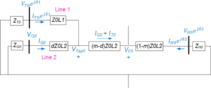
Zero-sequence network of the three-terminal line in Fig. 1 during a single or double line-to-ground fault
-
VG2,VH2,VT2 are the negative-sequence fault voltages at terminals G, H and T respectively
-
IG2,IH2,IT2 are the negative-sequence fault currents at terminals G,H and T respectively
-
VG0,VH0,VT0 are the zero-sequence fault voltages at terminals G, H and T respectively
-
IG0,IH0,IT0 are the zero-sequence fault currents at terminals G,H and T respectively
-
Z2L1 is the negative-sequence impedance of Line 1
-
Z2L2 is the negative-sequence impedance of Line 2
-
Z0L1 is the zero-sequence impedance of Line 1
-
Z0L2 is the zero-sequence impedance of Line 2

Since terminals G and T operate in parallel to feed the fault, VTap2 should be equal when calculated from either terminal. From this principle, ejδ1 can be solved as
In effect, this step calculates the phase angle mismatch between terminal G and terminal T measurements, and accordingly adjusts the phasors at terminal T by ejδ1.
2.1.2 Step 2: synchronize terminal H with terminals T and G
After the synchronization process in Step 1, the new negative-sequence voltage and current phasors at terminal T are VT2ejδ1 and IT2ejδ1, respectively, and at terminal G are VG2 and IG2, respectively. This step synchronizes the phasors at terminal H with the phasors at terminals G and T. For this purpose, a second synchronizing operator, ejδ2, is applied to the measurements at terminal H. The value of ejδ2 can be calculated from the fact that the negative-sequence voltage at the fault point, VF2, must be the same when calculated from either terminal G or H as
Therefore, ejδ2 is given by
At the end of this step, the voltage and current measurements at terminals T and H are synchronized with respect to those at terminal G.
2.1.3 Step 3: calculate the zero-sequence impedance of Line 2
To estimate the zero-sequence impedance of Line 2, the zero-sequence network during a single or double line-to-ground fault is shown in Fig. 3. The zero-sequence voltage at the fault point, VF0, can be calculated from terminal G and H as
Since VF0 is equal when calculated from either line terminal, equate the two equations in (5) to solve for Z0L2 as
2.1.4 Step 4: calculate the zero-sequence impedance of Line 1
To estimate the zero-sequence impedance of Line 1, Z0L1, calculate the zero-sequence voltage at the tap point, VTap0, from terminals G and T as
where VT0 is the zero-sequence fault voltages at terminal T. Because VTap0 from terminal G is equal to that from terminal T, we can use (7) to solve for Z0L1 as
In this way, Approach 1 is successful in validating the zero-sequence impedance of Line 1 and Line 2. If the actual fault location is not available, then an additional step (Step 0) must be performed to track down the exact fault location before applying the steps described above.
2.1.5 Step 0: identify the fault location
Before computing the distance to the fault, it is necessary to identify whether the fault is on Line 1 or on Line 2. The negative-sequence network shown in Fig. 2 is used for this purpose. When the fault is between terminal H and the tap point, VTap2 from the other two terminals are equal. Therefore, to identify the faulted section of the feeder, the approach consists of calculating VTap2 from each terminal as
The estimated |VTap2| from two of the terminals will be an exact match while |VTap2| from the third terminal will be different. The fault is expected to lie between that third terminal and the tap point. Next, apply one-ended fault location algorithm to the voltage and current waveforms at the third terminal and estimate the distance to the fault.
Figure 4 shows a flow diagram which summarizes Approach 1 for calculating the zero-sequence line impedance.

Flow diagram depicting Approach 1 for calculating zero-sequence line impedance of all the sections of a three-terminal line using data from all three terminals
2.2 Assumptions
Assumptions made by Approach 1 when estimating the zero-sequence impedances of Line 1 and Line 2 are summarized below:
1. Line 1 and Line 2 are homogeneous
2. Zero-sequence mutual coupling is absent
A transmission network is homogeneous when the local and remote source impedance have the same impedance angle as the transmission line. Assumption 1 is a reasonable assumption to make as local and remote source impedance angles are often close to that of the transmission line.
Zero-sequence mutual coupling arises when transmission lines are physically very close or parallel to each other. An example where zero-sequence mutual coupling could be present is when there are two sets of three-phase lines running on same towers. Though this configuration of lines is occasionally found in two-terminal transmission lines, it is highly unlikely and rare to have three-terminal transmission line with such a wire configuration that would have zero-sequence mutual coupling.
2.3 Approach 2 for estimating zero-sequence line impedance: data from two terminals
Although Approach 1 can successfully validate the zero-sequence impedance of three-terminal transmission lines, voltage and current waveforms from all the three terminals may not always be available. For this reason, this subsection develops a methodology that can use data from only two terminals to estimate the zero-sequence impedance of three-terminal lines. To illustrate the approach, consider the scenario shown in Fig. 1. Suppose that the measurements captured by digital relays at terminals G and H are available while measurements from terminal T are missing. The procedure to estimate the zero-sequence impedance of Line 1 and Line 2 in such a scenario is described below:
2.3.1 Step 1: estimate the negative-sequence current from terminal T
To estimate the negative-sequence fault current from terminal T, IT2, the negative-sequence network shown in Fig. 2 is used. The approach consists of calculating VTap2 from terminal G and terminal T as
where ZT2 is the negative-sequence source impedance of terminal T. Since VTap2 is equal when calculated from either terminal, IT2 can be estimated as
Note that since terminal G measurements are being used to estimate the fault current from terminal T, measurements of these two terminals are automatically synchronized.
2.3.2 Step 2: synchronize terminal H with terminals G and T
This step applies a synchronization operator, ejδ, to the terminal H measurements so as to align the measurements at this terminal with those at terminals G and T. The fact that VF2 is the same when calculated from terminals G and H is used to calculate the synchronization operator as
The new set of sequence voltage phasors at terminal H are VH1ejδ,VH2ejδ, and VH0ejδ. Similarly, the new set of current phasors at terminal H are IH1ejδ,IH2ejδ, and IH0ejδ.
2.3.3 Step 3: estimate the zero-sequence impedance of line 2
The zero-sequence line impedance of Line 2 is estimated from terminal H measurements using any zero-sequence line impedance estimation algorithm for two-terminal line which uses measurements from one terminal only [5, 11]. The algorithm to estimate the zero-sequence line impedance of a two-terminal line using data from only one terminal assumes that the fault resistance is zero and the fault location is known.
2.3.4 Step 4: estimate the zero-sequence current from terminal T
The zero-sequence voltage at the fault point, VF0, is the same when calculated from terminal G or terminal H. This principle is used to calculate the zero-sequence fault current contributed by terminal T, IT0, as
2.3.5 Step 5: estimate the zero-sequence impedance of line 1
The fact that VTap0 is the same when calculated from terminal G or terminal T is used to estimate the zero-sequence impedance of Line 1 as
Figure 5 shows a flow diagram which summarizes Approach 2 for calculating the zero-sequence line impedance.

Flow diagram depicting Approach 2 for calculating zero-sequence line impedance of all the sections of a three-terminal line using data from only two terminals
2.4 Assumptions:
Assumptions made by Approach 2 when estimating the zero-sequence line impedance are summarized below:
1. Line 1 and Line 2 are homogeneous
2. Fault location is known
3. Fault resistance is zero
4. Zero-sequence mutual coupling is absent
The assumptions that the transmission network is homogeneous and the absence of zero-sequence mutual coupling are same as that of Approach 1. Since Approach 2 has lesser data availability than Approach 1, further assumptions must be made to obtain the zero-sequence line impedance of the lines.
In utility/industry practice, the process of estimating the zero-sequence line impedance is an offline post fault analysis process using event reports recorded by the relay. The electric power utility performs a thorough investigation of the fault event as soon as the fault has occurred. As a result, it is expected that the utility identifies the fault location and hence, it is a reasonable assumption that the fault location is known while implementing the proposed algorithm.
It is highly unlikely to have a completely bolted fault where the fault resistance is exactly zero. However, it is a reasonable assumption to make when the fault resistance value is small and close to zero. Though not every short-circuit fault has a fault impedance value close to zero, the occurrence of this type of fault where the fault impedance is close to zero is relatively common in transmission lines. Such a scenario has also been demonstrated and analyzed using real-world field data in [5]. However, having to extract more information from less data requires us to make such an assumption.
3 Demonstration of estimation of zero-sequence impedance using a test case
This section demonstrates the efficacy of Approach 1 and Approach 2 in estimating the zero-sequence line impedance of a three-terminal line during a single line-to-ground fault. The system parameters used for the study are described below.
The three-terminal network shown in Fig. 1 was modeled in PSCAD simulation software [17]. The model was used to replicate actual short-circuit faults that occur on a transmission line and generate the corresponding voltage and current waveforms.
The positive- and zero-sequence source impedances at terminal G are ZG1 = 3.75 ∠86° Ω and ZG0 = 11.25 ∠86° Ω, respectively. The positive- and zero-sequence source impedances at terminal H are ZH1 = 12 ∠80° Ω and ZH0 = 36 ∠80° Ω, respectively. The positive- and zero-sequence source impedances at terminal T are ZT1 = 5 ∠83° Ω and ZT0 = 12 ∠83° Ω, respectively.
The distance between terminal G and the tap point is 6.21 miles. Line 2 is 18.64 miles long and has the same configuration as shown in Fig. 6. Shield wires S1 and S2 protect phase conductors A, B, and C from direct lightning strikes. The positive- and zero-sequence line impedances calculated using modified Carson’s model [18] at an earth resistivity value of 100 Ω-m are Z1L2 = 16.15 ∠70° Ω and Z0L2 = 34.87 ∠64° Ω, respectively. Line 1 is 6.21 miles long and also has the same configuration as Fig. 6. However, the earth resistivity was changed to 80 Ω-m. The positive- and zero-sequence line impedances are Z1L1 = 5.38 ∠70° Ω and Z0L1 = 11.55 ∠65° Ω, respectively.

Tower configuration of an actual 69-kV transmission line model used for demonstrating the proposed algorithms
When a bolted phase A-to-ground fault occurs at a distance of 13 miles from terminal G, monitors at terminals G, H, and T capture the voltage and current waveforms at 32, 64, and 128 samples per cycle, respectively. The waveforms are, therefore, not synchronized with each other.
For the test scenarios, the fundamental frequency magnitude and phase angle of the fault current and voltages were extracted using Fast Fourier Transform. To avoid inaccuracies due to transients and DC offset, a cycle with stable fault current is used. For this purpose, the third cycle after fault inception was chosen in the simulation results to estimate the zero-sequence line impedance. Fast Fourier Transform is a commonly used method to extract fundamental frequency components and filter out decaying DC offset [8, 19]. If the DC offset remains significant after the third cycle, more advanced filters [20, 21] can be used or appropriate fault cycle can be chosen to obtain accurate current and voltage measurements from fault records. This ensures that the error in determining the current and voltage phasors is minimized and hence the zero-sequence line impedance estimation will not be affected by it.
To assess the effectiveness of Approach 1, the fault location is assumed to be unknown. Following Step 0, the negative-sequence voltage magnitude at the tap point, |VTap2|, is calculated to be 4.05 kV from terminal G, 261.78 kV from terminal H, and 4.05 kV from terminal T. Since |VTap2| from terminals G and T are equal, the fault is expected to lie between terminal H and the tap point. Next, the simple reactance method [8] is applied to the measurements at terminal H and estimated the distance to the fault to be 13 miles from terminal G or 5.64 miles from terminal H. The next step is to synchronize the measurements at terminals T and H with those at terminal G, and estimate the zero-sequence impedances of Line 1 and Line 2. As seen from Table 1, the estimated line impedances match with those used in the simulation test case.
The magnitude and phase angle error were calculated as follows [6]:
Approach 2, on the other hand, uses the voltage and current waveforms captured at terminal G and terminal H, and assumes that the fault location is available. As seen from Table 2, the estimated line impedances are close to those used in the simulation. The magnitude error percentage of the estimated zero-sequence line impedance is less than 1% for both the approaches.
Although Approach 2 uses data from only two terminals to estimate the zero-sequence line impedance of all the sections of the three-terminal line, it requires the knowledge of source impedance parameters of the third terminal. For this purpose, the next section provides approaches to calculate the source impedance or the Thevenin impedance of the transmission network upstream from the monitoring location.
In [5], the transmission line, whose zero-sequence estimation was performed, was a two-terminal line whereas three-terminal transmission lines are analyzed in this paper. In a three-terminal transmission line, there is short-circuit current contribution from all three terminals unlike two-terminal transmission line where there is current contribution from only two terminals. Hence, the circuit explored, system equations and method of analysis are different compared to the algorithms presented in [5]. The data availability for a three-terminal line is also different from that of a two-terminal line. Moreover, there is a need to synchronize measurements from different terminals of the line based on data availability before estimating the zero-sequence line impedance. Furthermore, careful system analysis is required to calculate the zero-sequence impedance of both Line 1 and Line 2 as seen in the two approaches discussed above unlike having to estimate the zero-sequence impedance of only one line as in [5]. In addition to estimating the zero-sequence impedance of the lines, this paper also presents a method for estimating the Thevenin impedance of the transmission network upstream from the monition location using the same set of waveform data.
4 Estimating the Thevenin impedance of upstream network
Voltage and current waveforms captured by IEDs during a fault can be used to estimate the Thevenin impedance of the transmission network upstream from the monitoring location as illustrated in Fig. 7.

Concept of Thevenin impedance. The effect of the impedance of the upstream network can be emulated by replacing it with an equivalent impedance and this equivalent impedance is called Thevenin impedance
Figures 8, 9 and 10 represent the negative-, zero- and positive-sequence network respectively. The rest of the down stream network is represented as RDSN in Figs. 8, 9 and 10.

Negative-sequence network of a general transmission line network during an unbalanced fault

Zero-sequence network of a general transmission line network during a ground fault

Superposition theorem used to decompose the network into a prefault and a “pure” fault during a three-phase fault
The negative-sequence Thevenin impedance, ZG2, can be calculated from the negative-sequence network shown in Fig. 8 during an unbalanced fault as
In a similar manner, the zero-sequence source impedance, ZG0, can be calculated from the zero-sequence network in Fig. 9 during a ground fault as
The calculation of the positive-sequence source impedance, ZG1, on the other hand, is complicated by the presence of an internal generator voltage, EG, as shown in Fig. 10. As a workaround, the superposition principle is used to decompose the network into a prefault and “pure fault” network. Impedance ZG1 can be estimated from the “pure fault” network as
It should be noted that ZG1 is not assumed to be equal to ZG2 and is calculated separately using (19). This is because the positive-sequence impedance equals the negative-sequence impedance in static electrical components such as lines and transformers. However, the sequence impedances are not equal to each other in rotating machines.
5 Demonstration of estimation of Thevenin impedance of upstream network using a test case
To demonstrate the approach described in Section 4 for estimating the Thevenin impedance of the upstream network, the three-terminal line test case analyzed in Section 3 is used. The same fault scenario, a single line-to-ground (SLG) fault on phase A at a distance of 13 miles from terminal G with monitors at terminal G, H and T is used. The current and voltage waveforms recorded at terminal G are shown in Fig. 11.

Current and voltage waveforms recorded at terminal G. IA,IB and IC are the currents recorded in phases A, B and C respectively at terminal G. VA,VB and VC are the phase-ground voltages recorded in phases A, B and C respectively at terminal G
From the waveforms recorded by the relay at terminal G, the sequence voltage and current phasors before and during the fault are:
The above phasors are then used in (17)–(19) to calculate the Thevenin impedance of the upstream network of Terminal G. Table 3 presents the estimated Thevenin impedances at Terminal G.
As seen from Table 3, the estimated source impedances matched well with the actual impedances used in the simulation model. The magnitude error percentages of the estimated Thevenin impedances are less than 1%. The positive-sequence impedance shows a small deviation from the actual value. Most likely, the error stems from the constant current load model assumption in (19). Similarly, the Thevenin impedance can be estimated at Terminals H and T as well using sequence currents measured at their respective terminals.
The process of estimating the Thevenin impedance of the upstream network is done for each terminal of a transmission line. It requires data from only one terminal to estimate the Thevenin impedance of the upstream network of that terminal as shown in (17)–(19). It does not require data or information from other terminals of the line.
The calculation of Thevenin impedance or source impedance is done for the upstream network. Hence, the upstream Thevenin impedance is not affected by components downstream of the monitoring location. Therefore, the transmission line that is present after the monitor does not affect the Thevenin impedance of the upstream network.
6 Conclusion
This paper presents methods to estimate the zero-sequence line impedance of all the sections in a three-terminal transmission line using fault data from all three terminals as well as using data from only two terminals. When data from only two terminals are available, the algorithm requires source impedance data from the third terminal, assumes that the fault location is known and the fault resistance is zero. These assumptions are not required when data from all three terminals are available. The accuracy of the proposed methods are demonstrated using a test case. Both approaches produced accurate zero-sequence line impedance estimates when the assumptions were satisfied and the magnitude error percentage was less than 1%. Additionally, the paper also presented a technique for estimating Thevenin equivalent impedance of the transmission network upstream from the monitoring location. The efficacy of this method was demonstrated using a test case. The magnitude error percentage in estimating the Thevenin impedance was less than 1% in the test case. Hence, it can be concluded that the presented methods provide a reliable estimation of the zero-sequence impedance of the line and Thevenin impedance of the upstream network which can be used to verify relay settings.
References
Costello, D. (2008). Lessons learned analyzing transmission faults. In 2008 61st Annual Conference for Protective Relay Engineers, College Station, TX, (pp. 410–422).
Das, S., & Santoso, S. (2016). Utilizing relay event reports to identify settings error and avoid relay misoperations. In 2016 IEEE/PES Transmission and Distribution Conference and Exposition (T&D), Dallas, TX, (pp. 1–5).
Das, S., Navalpakkam Ananthan, S., Santoso, S. (2018). Relay performance verification using fault event records. Protection and Control of Modern Power Systems, 3(1), 22.
Ritzmann, D., Wright, P.S., Holderbaum, W., Potter, B. (2016). A method for accurate transmission line impedance parameter estimation. IEEE Transactions on Instrumentation and Measurement, 65(10), 2204–2213.
Das, S., Ananthan, S.N., Santoso, S. (2017). Estimating zero-sequence line impedance and fault resistance using relay data. IEEE Transactions on Smart Grid, PP(99), 1–1.
Amberg, A., Rangel, A., Smelich, G. (2012). Validating transmission line impedances using known event data. In 2012 65th Annual Conference for Protective Relay Engineers, College Station, TX, (pp. 269–280).
Zimmerman, K, & Costello, D (2010). Fundamentals and improvements for directional relays. In 2010 63rd Annual Conference for Protective Relay Engineers, College Station, TX, (pp. 1–12).
Das, S., Santoso, S., Gaikwad, A., Patel, M. (2014). Impedance-based fault location in transmission networks: theory and application. IEEE Access, 2, 537–557.
Sundaravaradan, N.A, & Reddy, M.J.B. (2018). How is earthing done?IEEE Potentials, 37(2), 42–46.
(2006). The complexity of protecting three-terminal transmission lines, System Protection and Control Task Force of the NERC Planning Commitee. Available: http://www.nerc.com/comm/PC/System%20Protection%20and%20Control%20Subcommittee%20SPCS%20DL/SPCTF-3TerminalLinesX091906.pdf. Accessed 4 Mar 2018.
Schweitzer III, E.O. (1990). A review of impedance-based fault locating experience. In 14th Annual Iowa-Nebraska System Protectection Seminar.
Santoso, S. (2009). Fundamentals of Electric Power Quality, Spring ed. Scotts Valley: CreateSpace.
Eriksson, L., Saha, M.M., Rockefeller, G.D. (1985). An accurate fault locator with compensation for apparent reactance in the fault resistance resulting from remote-end infeed. IEEE Transactions on Power Apparatus and Systems, PAS-104(2), 423–436.
Novosel, D., Hart, D., Hu, Y., Myllymaki, J. (1998). System for locating faults and estimating fault resistance in distribution networks with tapped loads. U.S. Patent 5839093.
Sharma, C., & Castellanos, F. (2006). Remote fault estimation and Thevenin impedance calculation from relays event reports. In 2006 IEEE/PES Transmission & Distribution Conference and Exposition: Latin America, Caracas, (pp. 1–7).
Sun, Y., Dai, C., Li, J. (2015). Thevenin equivalent circuit parameter estimation for the PCC upstream system. In 2015 5th International Conference on Electric Utility Deregulation and Restructuring and Power Technologies (DRPT), Changsha, (pp. 2299–2303).
PSCAD User’s Guide [Online] Available: https://hvdc.ca/uploads/knowledge_base/pscad_user_guide_v4_3_1.pdf?t=1462310124. Accessed 24 Sept 2018.
Kersting, W.H. (2012). Distribution System Modeling and Analysis, 3rd ed. Boca Raton: CRC Press.
Sundaram, A. (2006). Distribution fault location: field data and analysis. Palo Alto: EPRI. (1012438).
Min, K.W., & Santoso, S. (2017). DC offset removal algorithm for improving location estimates of momentary faults. IEEE Transactions on Smart Grid, PP(99), 1–1.
Zamora, A., Ramirez, J.M., Paternina, M.R.A., Vazquez-Martinez, E. (2015). Digital filter for phasor estimation applied to distance relays. IET General Transactions Distribution, 9(14), 1954–1963.
Author information
Authors and Affiliations
Contributions
SD and SNA had developed the algorithms, performed the analysis and drafted the manuscript. SS was the technical advisor and supervised the analysis and submission of the manuscript. All authors read and approved the manuscript.
Corresponding author
Ethics declarations
Competing interests
The authors declare that they have no competing interests.
Rights and permissions
Open Access This article is distributed under the terms of the Creative Commons Attribution 4.0 International License (http://creativecommons.org/licenses/by/4.0/), which permits unrestricted use, distribution, and reproduction in any medium, provided you give appropriate credit to the original author(s) and the source, provide a link to the Creative Commons license, and indicate if changes were made.
About this article

Cite this article
Das, S., Navalpakkam Ananthan, S. & Santoso, S. Estimating zero-sequence impedance of three-terminal transmission line and Thevenin impedance using relay measurement data. Prot Control Mod Power Syst 3, 36 (2018). https://doi.org/10.1186/s41601-018-0108-y
Received:
Accepted:
Published:
DOI: https://doi.org/10.1186/s41601-018-0108-y