Optimal operation modes of photovoltaic-battery energy storage system based power plants considering typical scenarios

Abstract

Recent advances in battery energy storage technologies enable increasing number of photovoltaic-battery energy storage systems (PV-BESS) to be deployed and connected with current power grids. The reliable and efficient utilization of BESS imposes an obvious technical challenge which needs to be urgently addressed. In this paper, the optimal operation of PV-BESS based power plant is investigated. The operational scenarios are firstly partitioned using a self-organizing map (SOM) clustering based approach. The revenue optimization model is adopted for the PV-BESS power plants to determine the optimal operational modes under typical conditions for a set of considerations, e.g. power generation revenue, assessing rewards/penalties as well as peak shaving/valley filling revenue. The solution is evaluated through a set of case studies, and the numerical result demonstrates the effectiveness of the suggested solution can optimally operate the BESS with the maximal revenue.

1 Introduction

The pursuit of low-carbon economy has significantly promoted the development of renewable energy across the world, particularly in China. Among the different renewable energy sources, photovoltaic (PV) has received much attention and the capacity of deployment is envisaged to quickly increase in the future [1]. It is well-known for the stochastic nature of the PV power generation [2,3,4,5]. Due to the fluctuations, there is a deviation between the predicted output and the actual output of PV power plant, which leads to the increase of the system rotation reserve capacity. Therefore, power dispatching agencies will assess the day-ahead power prediction accuracy of PV power plants, and PV power plants need to bear the corresponding assessment fees.

The BESS is capable of fast bidirectional regulation, and hence can be installed within the PV power plants for PV generation regulation [6, 7]. With the regulation and control of the BESS, the PV-BESS power plant can effectively restrain the fluctuation of PV power output, reducing the negative impact of photovoltaic power generation access to the grid. Furthermore, the deviation between actual output and predicted output of PV power can be reduced, which means the reserve costs of power grid enterprises and the assessment fees of the power plant will be reduced. Additionally, the potential of the BESS to participate in ancillary services can be fully excavated. Part of the BESS will be put into the auxiliary services such as peak shaving and valley filling, and a portion of additional economic benefits will be obtained. The combined generation of PV and BESS can provide a new solution to the grid connection of large-capacity PV power plants and is one of the future development directions.

Currently, the PV-BESS power generation is mainly based on demonstration projects. It is an important means to improve the economic efficiency of the PV-BESS power plants to take full use of the BESS and explore the feasible operation mode under the typical scenarios. A typical scenario of a PV-BESS power plant refers to a representative case with the typical temporal characteristics of PV power output embedded. The PV power generation is mainly affected by sunlight, and hence exhibit periodical and temporal characteristics [8]. To reduce the amount of calculation and maintain the objectivity of the analysis results, the PV power output of the PV-BESS power plant in the four seasons of the year can be divided into suitable typical scenarios.

There are few researches on operational mode of the PV-BESS power plants under typical scenarios. Some references about the typical scenarios analysis of wind farm and Microgrid, and the literatures about the economic operation control strategy and the optimal allocation of energy storage capacity can be referred to in this paper. Reference [9] presented a novel approach to planning distributed generation (DG) and distribution network frames based on a multi-scenario technique. A typical scene analysis method based on K means clustering algorithm was proposed in [10], and a typical scene set that reflects the characteristics of historical data within the computational cycle is formed. In [11], an annual time series production simulation model with large scale wind energy and solar power generation was developed based on timing sequence. In [12], the time series of wind power output curve and system load curve were studied based on the theory of time series analysis to calculate the capacity of wind power that the system can accept. In [13], aiming at minimizing the operation cost, an energy storage capacity optimization model considering the abandoned energy of wind power and the energy loss of the energy storage is constructed. In [14], with the minimum acquisition and replacement cost of energy storage system in the life cycle of wind farm as the optimization objective, the optimal allocation model of energy storage capacity is established. In [15], a practical and economical method for energy storage systems (ESS) configuration to stabilize the power fluctuation of distribution feeder lines was proposed on the basis of three types of filters.

In this paper, a typical scenarios segmentation method based on SOM clustering algorithm is proposed based on the historical power generation data of a PV power plant. Then with the optimization objective of maximizing economic returns, the optimal operation model of the PV-BESS under typical scenarios is established. The economic benefit in the model is the joint benefits of the power generation, the rewards or penalties of the assessment, and the benefit of the BESS from peak shaving and valley filling. Finally, on the basis of measured data of a PV power plant and the parameters of a demonstrative PV-BESS power plant, the operation modes of the PV-BESS power plant are established, which can provide guidance for the operation of the PV-BESS power plants.

2 Development of typical scenarios based on SOM clustering algorithm

2.1 Generation of forecasted PV power in typical scenarios of each season

In this paper, the daily generation of a PV power plant within a year is analyzed for four different seasons, i.e. spring, summer, fall and winter. The self-organizing map (SOM) clustering algorithm is employed to divide the PV output curves of each season into five categories. The clustering centers of each type are obtained as the forecasted PV output for each typical scenario.

The SOM neural network is an unsupervised competitive learning technique that can carry out the characteristic identification and clustering, e.g. load analysis and clustering [16,17,18]. SOM network consists of two layers neurons of input and output. Each neuron in the input layer is connected with neurons of the output layer through a variable weight, and the output neurons form a two-dimensional planar array.

In this work, the PV output vector P _pv,=[P _pv (1), P _pv (2), …, P _PV(n)] for in total 96 time slots is used as the input vector of SOM network, as illustrated in Fig. 1:

Fig. 1

PV output curve identification based on SOM clustering

Taking the spring as an example, the main steps of the generation of forecasted PV output in each typical scenario based on the SOM algorithm are as follows:

• (1) Determine the neural network structure. The number of neurons in the input layer is n = 96, and each neuron corresponds to a component of the input eigenvector. The number of output neurons is j = 1×5 = 5.

• (2) Network initialization. Set the random value of the [0,1] to the connection value w _nj (t) of the input element to the output element,n = 1, 2,…, 96;j = 1, 2, …, 5.

• (3) Select the PV output vector P _PV of one day in spring, provide it to the input layer and make the normalization:

$$ \overline{P_{pv}}=\frac{P_{pv}}{\left\Vert {P}_{pv}\right\Vert }=\frac{\left({P}_{pv}(1),{P}_{pv}(2),\cdots, {P}_{pv}(96)\right)}{\sqrt{{\left({P}_{pv}(1)\right)}^2+{\left({P}_{pv}(2)\right)}^2+\cdots +{\left({P}_{pv}(96)\right)}^2}}\kern0.75em $$

(1)

• (4) Calculate the Euclidean distance:

$$ {d}_j=\sqrt{\sum_{n=1}^{96}{\left(\overline{P_{pv}(n)}-{w}_{nj}\right)}^2},\kern0.5em j=1,2,\cdots, 5\kern1em $$

(2)

where, the neuron j* with the smallest distance is the winning neuron.

• (5) Adjust the connection weight vector. Update the connection vector of neurons within j*and its neighbourhood N _j* (t):

$$ {\displaystyle \begin{array}{l}\ {w}_{nj}\left(t+1\right)={w}_{nj}(t)+\eta (t)\left(\overline{P_{pv}}-{w}_{nj}(t)\right),\\ {}j=1,2,\cdots, 25\ \left(0<\eta (t)<1\right)\kern6em \end{array}} $$

(3)

where, η(t) is the variable learning speed, η(t) and N _j* (t) neighborhood decay with time.

• (6) Select the new day’s PV output data from step 3) to repeat the learning process until the daily PV output in the spring has been trained.

• (7) After the training, the output curves with the same winning neuron number are transformed into the same class.

• (8) Each clustering center obtained by formula (4) is used as the PV prediction output curve for each typical scenario Z _l , and Z _l  = {P _pv,1, P _pv,2, …, P _pv,l }.

$$ {P}_{pv\_ for}=\frac{1}{N_l}\sum_{i=1}^{N_l}{P}_{pv,i} $$

(4)

where, P _{pv_for} is the clustering center of Z _l , i.e. the forecasted PV output, P _{pv_for}  = [P _{pv_for} (1), P _{pv_for} (2), …, P _{PV_for} (k)], k = 1,2,…,96. N _l is the number of curves which contained by the Z _l , P _pv,i is the i-th PV output curve of in Z _l .

2.2 Generation of actual PV output in each typical scenario

Based on the five clustering results of each season’s PV output given in Section 2.1, all kinds of output curves are re-classified by SOM algorithm for more detailed clustering. The clustering centers of each type are obtained as the PV actual output P _{pv_act} for each typical scenario under different output conditions, and P _{pv_act}  = [P _{pv_act} (1), P _{pv_act} (2),…, P _{PV_act} (k)], k = 1,2,…,96. The main process is shown in Fig. 2.

Fig. 2

Generation of actual PV output in each typical scenario

3 Formulation of revenue optimization model

3.1 Objective functions

In this paper, the revenue of PV-BESS power plants in typical scenario is divided into three parts: power generation revenue, assessing rewards or penalties and peak shaving and valley filling revenue of the BESS. In different typical scenarios, the capacity of BESS for optimizing PV power and the capacity of BESS for peak shaving and valley filling are optimized to maximize the revenue of the PV-BESS based power plant.

3.1.1 Power generation revenue

The revenue of the PV-BESS power plant is mainly from the grid connected power generation. The electricity charge is settled in accordance with the regional unified photovoltaic benchmark price. The daily power generation revenue of the PV-BESS power plant can be expressed as:

$$ {R}_{elc}={\rho}_{pv}\cdot {Q}_{pv- bess} $$

(5)

$$ {\displaystyle \begin{array}{c}{Q}_{pv- bess}=\sum \limits_{k=1}^N{P}_{pv- bess}(k)\cdot \varDelta t\\ {}=\sum \limits_{k=1}^N\left({P}_{pv\_ act}(k)+{P}_{bess}^{opt}(k)\right)\cdot \varDelta t\end{array}} $$

(6)

where, R _elc is power generation revenue, ρ _PV is the unified photovoltaic benchmark price of the area, Q _pv-bess is daily generation, P _pv-bess (k) is the power of PV-BESS at sampling point, P _{pv_act} (k) is the PV power of sampling point, ${P}_{bess}^{opt}(k)$ is discharge power of the BESS at sampling point, ∆t is sampling time interval, N is the number of sampling points, N = 24/∆t.

3.1.2 Assessing rewards or penalties

After the photovoltaic power plant is connected to the power grid, the power generation will be assessed by the dispatching department according to the management measures. Take the detailed rules of the implementation of grid operation management for the north-west regional power plants in China as an example, according to Article No.31 [19], the deviation between the 96 points day-ahead forecasted PV power and the actual PV power should be less than 10%. If the deviation is less than 10%, the plant will be rewarded by 1000 yuan/(10⁴kWh) according to the integral electricity. If the deviation range is between 10% and 20%, the plant will be penalized by 1000 yuan/(10⁴kWh) according to the integral electricity. If the deviation is more than 20%, the plant will be penalized by 3000 yuan/(10⁴kWh) according to the integral electricity.

According to the regulation, the root mean square error (RMSE) is calculated as follows:

$$ {RMSE}_{pv}=\frac{\sqrt{\sum_{i=1}^n{\left({P}_{pv}(i)-{P}_{pv\_ for}(i)\right)}^2}}{C_{ap}\bullet \sqrt{n}}\times 100\% $$

(7)

where, RMSE _pv is the root mean square error between the day-ahead forecasted PV power and actual PV power (%), P _pv (i) is the actual PV power at i-th moment (kW), P _{pv_for} (i) is the forecasted PV power at i-th moment (kW), C _ap is the average capacity of generating units (kW), n is the number of moments traversed by the forecasting.

For PV-BESS power plants, the grid connected power is the sum of the PV power and BESS power, so the formula of RMSE above can be expressed as [20]:

$$ {\displaystyle \begin{array}{c}{RMSE}_{pv- bess}=\frac{\sqrt{\sum \limits_{i=1}^n{\left({P}_{pv- bess}(i)-{P}_{pv\_ for}(i)\right)}^2}}{C_{ap}\bullet \sqrt{n}}\times 100\%\\ {}=\frac{\sqrt{\sum \limits_{i=1}^n{\left({P}_{bess}^{opt}(i)+{P}_{pv\_ act}(i)-{P}_{pv\_ for}(i)\right)}^2}}{C_{ap}\bullet \sqrt{n}}\times 100\%\end{array}} $$

(8)

The assessing rewards or penalties of the PV-BESS power plant can be expressed as:

$$ {R}_{ass}={\alpha}_{ass}\cdot {Q}_{pv- bess} $$

(9)

where, R _ass is the assessing rewards or penalties (yuan), α _ass is the coefficient of the rewards or penalties (yuan/kWh). The value of α _ass can be set up according to the relevant contents of the assessing rules of the power grid enterprises in different regions.

3.1.3 Peak shaving and valley filling revenue of the BESS

The primary role of BESS in a PV-BESS power plant is to optimize the output of PV power generation system and reduce the deviation between the actual and forecasted PV output. While in actual operation, only the partial capacity of the BESS is needed by the optimization of PV power. The PV-BESS power plant can take the remaining BESS into the power grid to help cut peak and fill valley, charging with low electricity price in valley time, and discharging with high electricity price during peak time, to obtain some extra income [21].

The revenue of the BESS participating in peak shaving and valley filling can be calculated by the below formula:

$$ {R}_{tou}=\sum_{i=1}^{24}{\rho}_{tou}(i)\cdot {P}_{bess}^{tou}(i) $$

(10)

where, R _tou is the revenue of the BESS participating in peak shaving and valley filling (yuan), ρ _tou (i) is the time-of-use price during i-th period (yuan/kWh), Ptou bess(i) is the charging or discharging power of the BESS in i-th period (kW). At the same time, the BESS will only maintain a single charge or discharge state.

Based on the above analysis, the optimal objective functions of the revenue optimization model of PV-BESS power plants in typical scenario can be expressed as:

$$ \mathit{\operatorname{Max}}\kern0.5em {R}_{sum}={R}_{elc}+{R}_{ass}+{R}_{tou} $$

(11)

where, the R _sum is the revenue of the PV-BESS power plants.

3.2 Constraints

In the typical scenarios developed in this paper, the calculation of revenue should be consistent with the operation constraints of the PV-BESS power plant, as follows:

• (1) Power balance constraint of the whole system [22]

$$ {P}_{pv\_ act}(k)+{P}_{bess}^{opt}(k)={P}_{pv- bess}(k) $$

(12)

• (2) Power constraint of the BESS

$$ -{P}_{bess-\max}^{opt}\le {P}_{bess}^{opt}(k)\le {P}_{bess-\max}^{opt} $$

(13)

where, ${P}_{bess-\max}^{opt}$ is the maximum charge and discharge power of the BESS used to optimize PV power (kW).

• (3) State-of-Charge (SOC) constraint of the BESS [23]

The SOC of the BESS refers to the ratio of residual energy to total capacity. To prevent the overcharge and over discharge of the BESS, the SOC of the BESS should be bound up to the upper and lower limits.

$$ {SOC}_{bess.\min}^{opt}\le {SOC}_{bess}^{opt}(k)\le {SOC}_{bess.\max}^{opt} $$

(14)

where, ${\mathrm{SOC}}_{bess}^{opt}(k)$, ${\mathrm{SOC}}_{bess-\max}^{opt}(k)$ and ${\mathrm{SOC}}_{bess-\min}^{opt}(k)$ are respectively the SOC and the upper and lower limits at the k-th sampling point.

$$ {SOC}_{bess}^{opt}(k)={SOC}_{bess}^{opt}(0)-\frac{\sum_{i=1}^k{\eta}_{bess}{P}_{bess}^{opt}(i)\cdot \varDelta t}{E_{bess-\max}^{opt}} $$

(15)

where, ${\mathrm{SOC}}_{bess}^{opt}(0)$ is the initial state of the SOC (%), ${E}_{bess-\max}^{opt}$ is the rated capacity of the BESS used to optimize the PV output (kWh), η _bess is the charge and discharge efficiency of the BESS, which is set as 90% in this paper.

• (4) Capacity allocation constraints of the BESS

$$ 0\le {E}_{bess-\max}^{opt}\le {E}_{bess} $$

(16)

where, E _bess is the rated capacity of the whole BESS in the PV-BESS power plant.

4 Proposed algorithmic solution

In this paper, the joint benefit model of typical scenario for PV-BESS power plant is established, which mainly solves the following problems: by adjusting the capacity of the energy storage battery (${E}_{bess-\max}^{opt}$) to optimize the joint benefit (R _sum ) of the typical scenario making it can be maximized. The variables to be optimized are ${E}_{bess-\max}^{opt}$ and ${P}_{bess}^{opt}(k)$.

In a typical scenario, the PV prediction curve P _{pv_for} (k) and the actual curve P _{pv_act} (k) can be obtained from the analysis of the section 2. The solution of the model is as follows:

• (1) Enter calculation parameters P _pv-for (k) and P _{pv_act} (k).

• (2) Set the values of ${E}_{bess-\max}^{opt}$ and ${P}_{bess-\max}^{opt}$.

• (3) Let ${P}_{bess}^{opt}(k)$ as the input variable, calculate the minimum value of RMSE _PV-bess and the corresponding ${P}_{bess}^{opt}(k)$ using the genetic algorithm (GA).

• (4) Calculate the R _elc , the R _ass and the R _tou .

• (5) Calculate the R _sum of typical scenario for PV-BESS power plant.

• (6) Judge whether all values of the ${E}_{bess-\max}^{opt}$ are traversed; if so, proceed to the next step; otherwise, return to the step (2) and repeat steps (2) to (5).

• (7) Select the corresponding ${E}_{bess-\max}^{opt}$ as the optimal solution when the R _sum takes the maximum value.

• (8) The specific flow of model solving is shown in Fig. 3.

  Fig. 3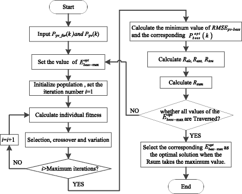

  

  The joint benefit model solving process of typical scenario for PV-BESS

For each typical scenario, the above model is used to calculate the optimal ${E}_{bess-\max}^{opt}(i)$ corresponding to each PV actual curve. The ${E}_{bess-\max}^{opt}$ is obtained by the formula (17):

$$ {E}_{bess-\max}^{opt}=\frac{\sum_{i=1}^3{E}_{bess-\max}^{opt}(i)\cdot {\eta}_{pv}(i)}{\eta_s} $$

(17)

Where, ${E}_{bess-\max}^{opt}(i)$ (i = 1,2,3) is the capacity of the BESS for optimizing PV output under the i-th PV actual curve for this typical scenario, η _pv (i) is the probability of the i-th actual PV curve, η _S is the probability of the typical scenario.

In summary, the forecasted PV output P _pv-for (k) and three types of actual PV output P _{pv_act} (k) in each scenario developed by the SOM are firstly employed as the calculation parameters. Then the Eopt bess-max(i) corresponding to the maximum value of R _sum with the P _pv-for (k) and i-th P _{pv_act} (k) is calculated based on GA. Finally, on the basis of ${E}_{bess-\max}^{opt}(i)$, η _pv (i) and η _S , the optimal ${E}_{bess-\max}^{opt}$ of each scenario can be calculated.

5 Case studies and numerical result

5.1 Data sources and system description

The object of this paper is the demonstration PV-BESS power plant built in Golmud District of Qinghai, China in 2016. In the PV-BESS power plant, the capacity of the PV generation units is 50 MW, the rated power of the energy storage system is 15 MW, and the rated capacity of the energy storage system is 18 MWh. Due to the short time of grid connection of the PV-BESS power plant, the historical data of PV power generation is from a 50 MW PV power plant in Haixi of Qinghai, China in 2012, and the sampling interval is 15 min. Some of the calculation parameters are shown in Table 1.

Table 1 Calculation parameters

The value of α _ass is set up according to the detailed rules of the implementation of grid operation management for the north-west regional power plants in China, which are shown in Table 2.

Table 2 Coefficients of the assessment rewards or penalties

According to the method of peak and valley time division in most provinces of China, the peak time is 08:00–12:00 and 17:00–21:00, the average time is 12:00–17:00 and 21:00–24:00, and the valley time is 00:00–08:00. The electricity tariff in the average time is the usual tariff, the electricity tariff in peak time is 50% higher than the usual tariff, and the electricity tariff in the valley time is 50% lower than the usual tariff.

5.2 Development of the typical scenarios

The historical data of PV power generation from a 50 MW PV power plant in Haixi of Qinghai, China in 2012 is employed to develop the typical scenarios of the PV-BESS power plant. The historical data sampling interval is 15 min, and there are 96 points in the daily generation power curve. First, the data is processed to kick out the bad data. Then the typical scenarios partition method based on SOM clustering algorithm proposed in this paper is applied to develop the typical scenarios of the PV-BESS power plant.

Typical scenarios of the four seasons of spring, summer, fall, winter and the output curves of representative scenario are shown in Figs. 4, 5, 6, 7. There are five typical scenarios in each season: (a) ~ (e), and the output curves of representative scenario of each season include the predicted output curve: PV_for, and three different actual output curves: PV1, PV2 and PV3. PV_for is the clustering center curve of the representative scenario. Due to the influence of the sunlight, part of the 96 sampling data of the PV output curve is zero. For ease of analysis, only the sampling data between 8:00 to 20:00 of the typical scenarios are shown. The distribution probability of the typical scenarios and three actual PV output curves in each typical scenario are shown in Fig. 8.

Fig. 4

Typical scenarios and the output curves of representative scenario in spring

Fig. 5

Typical scenarios and the output curves of representative scenario in summer

Fig. 6

Typical scenarios and the output curves of representative scenario in fall

Fig. 7

Typical scenarios and the output curves of representative scenario in winter

Fig. 8

The distribution probability of typical scenarios in the four seasons of the year (%)

The clustering results above show that the typical scenarios of photovoltaic power generation in different seasons are divided into 5 types, and the clustering center of each typical scenario is regarded as the forecasted PV power. The PV output curves included in each typical scenario are clustered into 3 types, the clustering centers are the three typical actual PV output. As the weather condition is the main factor of PV power generation, each typical scenario reflects the influence of different weather conditions on the PV output to a certain extent. For example, the 5 typical scenarios in summer correspond to sunny all day, sunny in the morning while cloudy in the afternoon, cloudy in the morning while sunny in the afternoon, cloudy all day and overcast all day.

5.3 Optimal operation mode under typical scenarios

On the basis of cluster analysis of typical scenarios of PV-BESS power plants in different seasons of the year, taking the typical scenarios (a) and (d) as an example, the process of the development of the optimal operation mode of PV-BESS in typical scenarios applying the revenue optimization model is analyzed in detail. Figs. 9 and 10 and Table 3 are the results of the model optimization. The ${E}_{bess}^{opt}-{R}_{sum}$ curves under different actual PV output in the typical scenario (a) and (d) of summer are shown below.

Fig. 9

The relationship curve of ${E}_{bess}^{opt}-{R}_{sum}$ under different actual PV output in the typical scenario (a) of summer

Fig. 10

The relationship curve of ${E}_{bess}^{opt}-{R}_{sum}$ under different actual PV output in the typical scenario (d) of summer

Table 3 The operation mode and revenue of the typical scenario (a) and (d) of summer

The following conclusions can be drawn from Figs. 9 and 10 and Table 3:

• (1) In the same typical scenario, under different actual PV power, the operation mode of the PV-BESS power plant is different, while the trends in the relationship curve of ${E}_{bess}^{opt}-{R}_{sum}$ are the same. This is primarily because that in the same typical scenario, the weather conditions are the same, the change trends of the PV power are the same, and the accuracies of the day-ahead PV power forecasting are similar.

• (2) In different typical scenarios, the optimal operation modes of PV-BESS power plant are different. Because in different typical scenarios, the weather conditions are different, the change trends of the PV power are different, and the accuracies of the day-ahead PV power forecasting are different. For example, in the typical scenario (a) of summer, the weather condition is sunny all day, and the fluctuation of sunlight is small, so the accuracy of the day-ahead PV power forecasting is high. While the weather condition of the typical scenario (d) of summer is cloudy all day, and the fluctuation of sunlight is large, so the accuracy of the day-ahead PV power forecasting is low.

• (3) The main factor that affects the operation mode optimization of typical scenarios of PV-BESS power plants is the assessing rewards or penalties. The purpose of developing the operation modes of PV-BESS power plants is to reduce the deviation between the day-ahead forecasted and the actual PV power by the configuration of the BESS to regulate the PV output, so the assessing penalties can be reduced, or the assessing rewards can be obtained.

The operation modes and expected revenue of the PV-BESS power plant in the typical scenarios in four seasons of the year are shown in Table 4.

Table 4 The operation modes and expected revenue of the PV-BESS power plant in the typical scenarios

Table 4 indicates that in different typical scenarios, the demand of the PV-BESS power plant for the capacity and power of the BESS is different. Based on the detailed analysis of photovoltaic power generation in typical scenarios, the BESS can be allocated rationally, which means the operation modes can be developed to guide the operation of the PV-BESS power plant and help it gain greater economic benefits.

5.4 Revenue comparison between the optimal typical scenario operation modes and the current operation modes

In the current operation mode of the PV-BESS power plant, the whole BESS is used to optimize the PV output to reduce the deviation between the day-ahead forecasted PV power and the actual PV power. The revenue of the PV-BESS power plant between the optimal typical scenario operation modes and the current operation modes are compared. The comparison results of the revenue in the twenty typical scenarios in spring, summer, fall and winter are shown in Fig. 11.

Fig. 11

Revenue comparison between the optimal typical scenario operation modes and the current operation modes

Fig. 11 indicates that compared with the current operation mode, the optimal typical scenario operation modes established in this paper can help the PV-BESS power plant to obtain higher expected economic benefits. In the current operation mode, the annual expected revenue of the PV-BESS power plant is 88.609 million yuan. The annual expected revenue of the PV-BESS power plant with the optimal typical scenario operation modes is 90.812 million yuan, with additional revenue of 2.203 million yuan.

6 Conclusions

In this paper, the PV power output curves of the PV-BESS power plant are classified into different typical scenarios based on the analysis of the historical data of PV power generation. Then the optimization model for maximal revenue of the PV-BESS power plants in typical scenarios considering power generation revenue, assessing rewards or penalties and peak shaving and valley filling revenue of the BESS is established. On the basis of this model, the feasible operation models in different typical scenarios of the PV-BESS power plant are discussed. The results of the case studies indicate that applying the typical scenarios analysis method and revenue optimization model, the BESS of the PV-BESS power plant can be allocated rationally to develop feasible operation modes, which can provide guidance for the operation of the PV-BESS power plant.

References

Ravikumar, D., Wender, B., Seager, T. P., et al. (2017). A climate rationale for research and development on photovoltaics manufacture[J]. Appl Energy, 189, 245–256.
Wu, K., Zhou, H., An, S., et al. (2015). Optimal coordinate operation control for wind–photovoltaic–battery storage power-generation units [J]. Energy Convers Manag, 90, 466–475.
Barbieri, F., Rajakaruna, S., & Ghosh, A. (2017). Very short-term photovoltaic power forecasting with cloud modeling: A review[J]. Renew Sust Energ Rev, 75, 242–263.
Shivashankar, S., Mekhilef, S., Mokhlis, H., et al. (2016). Mitigating methods of power fluctuation of photovoltaic (PV) sources–A review[J]. Renew Sust Energ Rev, 59, 1170–1184.
Shin, S. S., Oh, J. S., Jang, S. H., et al. (2017). Active and Reactive Power Control of ESS in Distribution System for Improvement of Power Smoothing Control[J]. Journal of Electrical Engineering & Technology, 12(3), 1007–1015.
Alam, M. J. E., Muttaqi, K. M., & Sutanto, D. (2014). A Novel Approach for Ramp-Rate Control of Solar PV Using Energy Storage to Mitigate Output Fluctuations Caused by Cloud Passing[J]. IEEE Transactions on Energy Conversion, 29(2), 507–518.
Li, X., Hui, D., & Lai, X. (2013). Battery Energy Storage Station (BESS)-Based Smoothing Control of Photovoltaic (PV) and Wind Power Generation Fluctuations[J]. IEEE Transactions on Sustainable Energy, 4(2), 464–473.
Wang, T., Bi, T., Wang, H., et al. (2015). Decision tree based online stability assessment scheme for power systems with renewable generations[J]. CSEE Journal of Power and Energy Systems, 1(2), 53–61.
Gao, Y., Hu, X., Yang, W., Liang, H., Li, P. (2017). Multi-Objective Bilevel Coordinated Planning of Distributed Generation and Distribution Network Frame Based on Multiscenario Technique Considering Timing Characteristics. IEEE Transactions on Sustainable Energy, 8(4), 1415–1429.
Ding, M., Xie, J., Pan, H., et al. (2017). Typical sequential scenario analysis method for economic operation of microgrid [J]. Automation of Electric Power Systems, 37(4), 11–16.
Zhao, X., Wu, L., & Zhang, S. (2013). Joint environmental and economic power dispatch considering wind power integration: Empirical analysis from Liaoning Province of China[J]. Renew Energy, 52, 260–265.
Pan, Y., Mei, S., Liu, F., et al. (2016). Admissible Region of Large-Scale Uncertain Wind Generation Considering Small-Signal Stability of Power Systems[J]. IEEE Transactions on Sustainable Energy, 7(4), 1611–1623.
Nguyen, C. L., Chun, T. W., & Lee, H. H. (2013). Determination of the optimal battery capacity based on a life time cost function in wind farm[C]//Energy Conversion Congress and Exposition (ECCE), 2013 IEEE, IEEE (pp. 51–58).
Wu, J., Zhang, B., Li, H., et al. (2014). Statistical distribution for wind power forecast error and its application to determine optimal size of energy storage system[J]. Int J Electr Power Energy Syst, 55(2), 100–107.
Cao, M., Xu, Q., Bian, H., et al. (2016). Research on configuration strategy for regional energy storage system based on three typical filtering methods[J]. IET Generation, Transmission & Distribution, 10(10), 2360–2366.
Du, L., Restrepo, J. A., Yang, Y., et al. (2013). Nonintrusive, self-organizing, and probabilistic classification and identification of plugged-in electric loads[J]. IEEE Transactions on Smart Grid, 4(3), 1371–1380.
McLoughlin, F., Duffy, A., & Conlon, M. (2015). A clustering approach to domestic electricity load profile characterisation using smart metering data[J]. Appl Energy, 141, 190–199.
Moeini, A., Darabi, A., Rafiei, S. M. R., et al. (2011). Intelligent islanding detection of a synchronous distributed generation using governor signal clustering[J]. Electr Power Syst Res, 81(2), 608–616.
Detailed rules of the implementation of grid operation management for the north-west regional power plants in China. Northwest Regulation Bureau of National Energy Bureau.http://news.bjx.com.cn/html/20161114/788693.shtml. Accessed on 11 Aug 2017.
GB/T 19964–2012. (2012). Technical regulations for photovoltaic power station access to power systems [S]. BeiJing: Standards Press of China.
Yang, Y., Li, H., Aichhorn, A., et al. (2014). Sizing strategy of distributed battery storage system with high penetration of photovoltaic for voltage regulation and peak load shaving[J]. IEEE Transactions on Smart Grid, 5(2), 982–991.
Mojica-Nava, E., Macana, C. A., & Quijano, N. (2014). Dynamic population games for optimal dispatch on hierarchical microgrid control [J]. IEEE Transactions on Systems, Man, and Cybernetics: Systems, 44(3), 306–317.
Zhao, B., Zhang, X., Chen, J., et al. (2013). Operation optimization of standalone microgrids considering lifetime characteristics of battery energy storage system[J]. IEEE Transactions on Sustainable Energy, 4(4), 934–943.
Author information
Authors and Affiliations
Contributions
FX carried out the main research tasks and wrote the full manuscript, and YG proposed the original idea, analyzed and double-checked the results and the whole manuscript. WY, QY, YS and YS contributed to data processing and to writing and summarizing the proposed ideas, while HL and PL provided technical and support throughout. All authors read and approved the final manuscript.
Corresponding author
Ethics declarations
Competing interests
The authors declare that they have no competing interests.
Rights and permissions
Open Access This article is distributed under the terms of the Creative Commons Attribution 4.0 International License (http://creativecommons.org/licenses/by/4.0/), which permits unrestricted use, distribution, and reproduction in any medium, provided you give appropriate credit to the original author(s) and the source, provide a link to the Creative Commons license, and indicate if changes were made.
About this article
Cite this article
Gao, Y., Xue, F., Yang, W. et al. Optimal operation modes of photovoltaic-battery energy storage system based power plants considering typical scenarios. Prot Control Mod Power Syst 2, 36 (2017). https://doi.org/10.1186/s41601-017-0066-9
Received:
Accepted:
Published:
DOI: https://doi.org/10.1186/s41601-017-0066-9